MLE for Bernoulli Parameters

Hello! Welcome back to our series on the theoretical foundations of AI.

In the previous lesson, we formulated the principle of Maximum Likelihood Estimation (MLE), establishing it as a powerful and theoretically grounded method for finding estimators. We learned that MLE chooses the parameters that make our observed data most probable, and that this is equivalent to minimizing the KL Divergence between our model and the true data-generating distribution.

Today, we move from principle to practice. Your learning outcome is to derive the MLE for the parameter of a Bernoulli distribution. This will be our first complete application of the MLE "recipe":

1. Formulate the likelihood and log-likelihood functions.
2. Use calculus to find the parameter value that maximizes this function.
3. Verify that this value is indeed a maximum.

This exercise will solidify your understanding of the MLE process and yield a result that is both mathematically sound and highly intuitive.

1. The Bernoulli Distribution and its Likelihood

Let's start by recalling the Bernoulli distribution. It models a single trial with two outcomes, typically labeled 1 (success) and 0 (failure). The probability of success is given by a single parameter, which we'll call $p$.

The Probability Mass Function (PMF) for a Bernoulli-distributed random variable $X$ can be written compactly as:
$P(X=x|p)=p^x(1-p{)}^{1-x},\text{for }x\in \{0,1\}$
You can verify that if you plug in $x=1$, you get $p$, and if you plug in $x=0$, you get $1-p$.

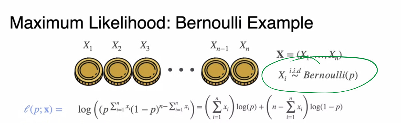
Now, assume we have a dataset $D=\{x_1,x_2,\dots ,x_n\}$ consisting of $n$ independent and identically distributed (i.i.d.) Bernoulli trials. Our task is to find the MLE for the parameter $p$.

The following video provides a clear, step-by-step derivation of the likelihood and log-likelihood functions for this exact scenario.

Summarizing the Log-Likelihood

As demonstrated in the video, the derivation proceeds as follows:

1. Likelihood Function: Due to the i.i.d. assumption, the likelihood is the product of the individual probabilities:
   $L(p;D)={\prod }_{i=1}^n{p}^{x_i}(1-p{)}^{1-x_i}$
   Using exponent rules, this simplifies to:
   $L(p;D)=p^{{\sum }_{i=1}^n{x}_i}(1-p{)}^{n-{\sum }_{i=1}^n{x}_i}$

2. Log-Likelihood Function: Taking the natural logarithm transforms the product and exponents:
   $l(p;D)=\log (L(p;D))=\left({\sum }_{i=1}^n{x}_i\right)\log (p)+\left(n-{\sum }_{i=1}^n{x}_i\right)\log (1-p)$

To make this expression cleaner, let's define $N_1={\sum }_{i=1}^n{x}_i$ as the total number of successes (heads, 1s) and $N_0=n-N_1$ as the total number of failures (tails, 0s). The log-likelihood function is then:
$l(p;D)=N_1\log (p)+N_0\log (1-p)$

2. Deriving the Maximum Likelihood Estimate

Now that we have our objective function, $l(p;D)$, we need to find the value of $p$ that maximizes it. Since this is a differentiable function with respect to $p$, we can use calculus. This involves finding the derivative, setting it to zero to find critical points, and using the second derivative to confirm that our critical point is a maximum.

This process connects directly to the unconstrained optimization theory we covered in Module 4.

The following text provides a concise, formal derivation of the MLE for the Bernoulli parameter, which you can use as a reference.

Let's walk through the steps of the derivation together.

Step 1: Differentiate the Log-Likelihood

We take the first derivative of $l(p;D)$ with respect to $p$:

$$\frac{d}{dp}l(p;D)=\frac{d}{dp}[N_1\log (p)+N_0\log (1-p)]$$

Using the rules for differentiating logarithms ($\frac{d}{dx}\log (x)=\frac{1}{x}$) and the chain rule for the second term, we get:

$$\frac{d}{dp}l(p;D)=\frac{N_1}{p}+\frac{N_0}{1-p}\cdot (-1)=\frac{N_1}{p}-\frac{N_0}{1-p}$$

Step 2: Set Derivative to Zero and Solve

To find the critical point, we set the derivative to zero and solve for $p$:

$$\frac{N_1}{p}-\frac{N_0}{1-p}=0$$ $$\frac{N_1}{p}=\frac{N_0}{1-p}$$

Now, we cross-multiply:

$$N_1(1-p)=N_{0}p$$ $$N_1-N_{1}p=N_{0}p$$ $$N_1=N_{0}p+N_{1}p=(N_0+N_1)p$$

Since $N_0+N_1=n$ (the total number of trials), we have:

$$N_1=np$$

Solving for $p$ gives us the maximum likelihood estimate, ${\hat{p}}_{MLE}$:

$${\hat{p}}_{MLE}=\frac{N_1}{n}=\frac{{\sum }_{i=1}^n{x}_i}{n}$$

This result is remarkably intuitive: the MLE for the probability of success in a series of Bernoulli trials is simply the proportion of successes observed in the data, also known as the sample mean.

Test your understanding!

You flip a coin, which you suspect might be biased, 100 times. You observe 65 heads and 35 tails. What is the maximum likelihood estimate for the probability of this coin landing on heads?

Show answer

The number of trials is $n=100$. The number of successes (heads) is $N_1=65$.
The MLE for the probability of heads, ${\hat{p}}_{MLE}$, is the proportion of successes:
${\hat{p}}_{MLE}=\frac{N_1}{n}=\frac{65}{100}=0.65$
This aligns perfectly with our intuition. The most likely value for the coin's bias is the one that reflects the frequency we observed.

Step 3: Verify the Maximum with the Second Derivative Test

To be mathematically rigorous, we must confirm that this critical point corresponds to a maximum, not a minimum or saddle point. We do this by checking the sign of the second derivative.

Let's continue with the video, which explicitly calculates the second derivative and analyzes its sign to complete the proof.

As the video explained, the second derivative of the log-likelihood is:

$$\frac{d^2}{d{p}^2}l(p;D)=\frac{d}{dp}\left[\frac{N_1}{p}-\frac{N_0}{1-p}\right]=-\frac{N_1}{p^2}-\frac{N_0}{(1-p{)}^2}$$

Let's analyze this expression:

• $N_1$ and $N_0$ are counts, so they are non-negative ($\ge 0$).
• For any valid probability $p\in (0,1)$, the terms $p^2$ and $(1-p{)}^2$ are strictly positive.
• Therefore, $\frac{N_1}{p^2}$ and $\frac{N_0}{(1-p{)}^2}$ are both non-negative.

The second derivative is $-\left(\frac{N_1}{p^2}+\frac{N_0}{(1-p{)}^2}\right)$. As long as we have at least one success and one failure (so the problem is non-trivial), this expression is strictly negative. A negative second derivative confirms that the function is concave and our critical point ${\hat{p}}_{MLE}=N_1/n$ is a local maximum. For a concave function, this local maximum is also the unique global maximum.

Conclusion

Congratulations! You have successfully completed your first end-to-end derivation of a Maximum Likelihood Estimator. We applied the general principle learned in the last lesson to a concrete distribution and, using calculus, arrived at a simple and intuitive result.

Key Takeaways:

• The log-likelihood function for $n$ i.i.d. Bernoulli trials with parameter $p$ is $l(p)=N_1\log (p)+N_0\log (1-p)$, where $N_1$ and $N_0$ are the counts of successes and failures.
• By differentiating, setting to zero, and solving, we found the MLE for the Bernoulli parameter: ${\hat{p}}_{MLE}=\frac{N_1}{n}$. This is simply the sample mean, or the proportion of successes.
• The second derivative test confirms that this solution maximizes the log-likelihood function, fulfilling the requirement for mathematical rigor.

Preview of the Next Lesson:
We have now applied MLE to a discrete distribution. In the next lesson, we will tackle a continuous one: the Gaussian (or Normal) distribution. You will derive the MLE for the parameters ($\mu$ and ${\sigma }^2$) of a Gaussian distribution. This will introduce a new challenge: optimizing a function with respect to multiple parameters simultaneously, which will require the use of partial derivatives.