Recommended resources
The freely available resources this lesson will direct you to.
Hello! Welcome to our lesson on the predictive power of the -expansion.
In our last session, we derived the first-order corrections to several critical exponents by analyzing the Wilson-Fisher fixed point in dimensions. We found results like and . While these calculations are performed for an infinitesimally small , their real test lies in their ability to describe physical systems, most notably those in three dimensions, where .
Today, we will address this head-on. Our goal is to compare the predictions of the -expansion for with the highly precise numerical results for the 3D Ising model. This comparison will not only quantify the success of our first-order approximation but also lead us to a deeper understanding of the nature of perturbative expansions in field theory and the sophisticated techniques used to extract physical meaning from them.
1. A First Look: Comparing First-Order Predictions with 3D Ising Values
Let's begin by assembling the first-order predictions from the -expansion and setting . The following resource conveniently summarizes these results.
Tutorial 4: The Renormalization Group and the Ising Model
This short excerpt from a tutorial on the renormalization group lists the critical exponents for the Ising model to first order in ε. It provides the formulae we will use for our initial comparison.
Please read the final paragraph on page 28, which lists the first-order expressions for α, β, γ, δ, η, and ν.
Now, let's compare these theoretical predictions with the best-known values for the 3D Ising model, which are obtained from demanding numerical methods like Monte Carlo simulations and the conformal bootstrap. The table below presents this comparison, including the classical mean-field values for context.
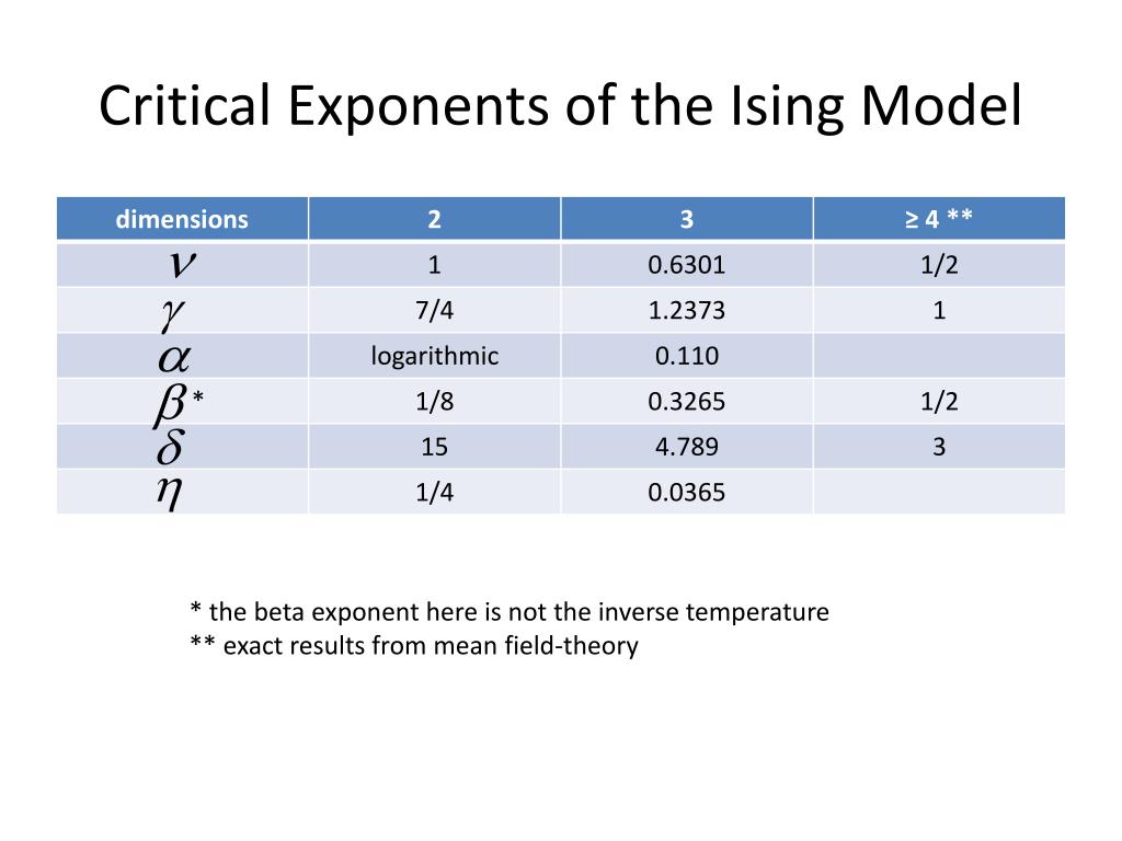
Here is a side-by-side comparison for :
| Exponent | Mean-Field Theory | 1st-Order -Expansion () | "Exact" Numerical Value (d=3) |
|---|---|---|---|
| 0 (discontinuity) | 0.110 | ||
| 0.5 | 0.326 | ||
| 1.0 | 1.237 | ||
| 3.0 | 4.790 | ||
| 0 | 0.036 | ||
| 0.5 | 0.630 |
Note: We previously stated . The leading term, which requires a two-loop calculation, is . Even with this, the prediction is off by a factor of two.
Observations:
- For every single exponent, the first-order -expansion provides a value that is significantly closer to the true value than mean-field theory.
- The prediction for is remarkably accurate, off by only about 2%.
- Other predictions, like for and , are qualitatively correct but have errors of about 6-8%.
- The predictions for and are the least accurate at this order.
The conclusion is clear: the -expansion works surprisingly well, even for a value as large as . However, to achieve the high precision seen in modern physics, we must go beyond this simple first-order analysis.
2. The Nature of the -Expansion: Asymptotic Series
One might assume that the path to higher precision is simply to calculate more terms in the expansion (e.g., , , etc.). However, there is a fundamental subtlety: the -expansion is an asymptotic series, not a convergent one. This means that after a certain point, adding more terms actually makes the approximation worse.
This divergence is not just a mathematical quirk; it has a deep physical origin. The following reading explains this by considering what happens in theory when the coupling constant is negative.
Benchmarking the Ising universality class in 3 ≤ d < 4 dimensions
To understand why the perturbative expansion diverges, we will read an excerpt from a state-of-the-art research paper that benchmarks the Ising universality class. This section explains the asymptotic nature of the series and its connection to instantons.
Please read Section 3.1, 'Warm-up analysis of the anomalous dimensions γσ' (pages 9-11). Focus on the discussion around equations (6) and (7). The key idea is that the number of Feynman diagrams grows factorially, causing the series to have a zero radius of convergence.
As the paper explains, the number of Feynman diagrams at -th order grows like . This factorial growth overpowers any term for non-zero coupling , leading to a divergent series. The physical reason is that for , the potential is unbounded from below, making the vacuum unstable. The path integral is dominated by non-perturbative "instanton" configurations, and their contribution is what the perturbation series is trying—and failing—to capture.
This leads to a classic behavior for asymptotic series: for a given value of , there is an optimal number of terms to include. The error decreases as you add the first few terms, but then hits a minimum and starts to increase. The paper you just read illustrates this perfectly in its Figure 5, which shows that for (), the 2- and 3-loop expansions are decent, but by 4-loops and beyond, the series rapidly diverges from the correct value.
3. Taming the Divergence: Borel Resummation
How can we extract high-precision information from a divergent series? The answer lies in a powerful technique called resummation. The most common method in this context is Borel resummation.
The core idea is to transform the original divergent series into a new one that converges.
- Borel Transform: Take the original series for an exponent . The factorial growth is in the coefficients . The Borel transform creates a new function, , by dividing each coefficient by : . This new series has a finite radius of convergence.
- Analytic Continuation: The function is then analytically continued outside its initial radius of convergence. This is the most technical and assumption-laden step.
- Inverse Transform: The resummed value is recovered by computing the integral .
While the details are highly technical, the conceptual point is that this procedure "tames" the factorial divergence and allows for the extraction of a meaningful, precise physical prediction.
4. The State of the Art: A Modern Comparison
With an understanding of resummation, we can now appreciate the comparison between the -expansion and other cutting-edge methods. The paper we've been examining provides a definitive summary.
Benchmarking the Ising universality class in 3 ≤ d < 4 dimensions
We will now study the part of the paper that summarizes the results for d=3 from various methods. This will be the capstone of our comparison.
Please examine Table 4 on page 18 and the accompanying Figures 11 and 12 on page 17. This table compiles the modern values for the scaling dimensions of the key operators in the 3D Ising model. Notice the incredible agreement between different methods like Bootstrap, Monte Carlo, and the 'Borel resummed epsilon expansion'.
Table 4 from the paper is a testament to the power of modern theoretical physics. It compares the scaling dimensions of the spin operator (, related to ) and the energy operator (, related to ). These are related to the standard critical exponents and by:
Test your understanding!
Using the values from "Borel resummed epsilon expansion" in Table 4 for , calculate the critical exponents and . How do they compare to the "Monte Carlo" values?
Given:
- From Table 4, "Borel resummed epsilon expansion":
- From Table 4, "Monte Carlo":
Show answer
Let's do the calculation for the resummed -expansion:
Now for Monte Carlo:
The agreement is remarkable. The resummed -expansion predicts values that are consistent with the extremely precise Monte Carlo results to within the stated error bars. This shows how a properly treated divergent series can yield phenomenally accurate predictions.
Conclusion
Today we have seen the -expansion in its full context, from a simple first-order approximation to a high-precision computational tool.
Key Takeaways:
- The first-order -expansion for () provides a significant qualitative and semi-quantitative improvement over mean-field theory.
- The expansion is an asymptotic series due to factorial growth in the number of Feynman diagrams, a consequence of the theory's instability for negative coupling.
- Advanced techniques like Borel resummation are required to extract precise, convergent results from this divergent series.
- When properly resummed, the -expansion yields critical exponents for the 3D Ising model that are in stunning agreement with the most precise values from non-perturbative methods like conformal bootstrap and Monte Carlo simulations.
Preview of the Next Lesson:
Having established the power and subtleties of the RG approach for a single universality class, we will next explore how the RG framework describes crossover phenomena. We will investigate how a system's behavior can "flow" from being described by one fixed point (e.g., Gaussian) to another (e.g., Wilson-Fisher) as a physical parameter, like temperature or interaction range, is varied. This will further highlight the dynamic and powerful picture that the renormalization group paints of the world of critical phenomena.