From φ⁴ to O(n): Describing Multi-Component Order Parameters

Hello! Welcome to your next lesson.

In our previous session, we saw how the renormalization group (RG) framework provides a powerful lens for understanding crossover phenomena. We focused on the scalar ${\varphi }^4$ theory, seeing how RG flows connect different fixed points and explain the transitions between, for example, mean-field and Ising-like critical behavior. That theory, with its single-component order parameter $\varphi$, is perfect for describing systems like the Ising model or the liquid-gas transition.

However, many of the most interesting systems in condensed matter physics possess order parameters with a richer structure—they are vectors or complex fields, not simple scalars. Think of a Heisenberg magnet where spins can point anywhere in 3D space, or a superfluid described by a complex order parameter.

Today, we will generalize the ${\varphi }^4$ theory to the O(n) model to describe systems with n-component order parameters. This generalization is a cornerstone of modern statistical field theory. We will:

1. Construct the appropriate Hamiltonian for an n-component vector order parameter.
2. Identify the physical systems corresponding to different values of $n$.
3. Analyze the RG flow equations for this generalized model and see how the universal aspects of critical phenomena depend on $n$.

This step is crucial for expanding our framework to a much wider array of physical problems and for understanding what ingredients—dimensionality, symmetry—truly define a universality class.

1. From Scalar to Vector: The O(n) Model

The generalization from a scalar field $\varphi (x)$ to a vector field is conceptually straightforward. We simply replace the single field with an n-component vector:

$$\vec{\varphi }(x)=({\varphi }_1(x),{\varphi }_2(x),\dots ,{\varphi }_n(x))$$

The key challenge is to construct a Landau-Ginzburg-Wilson Hamiltonian (or action) that respects the underlying symmetry of the system. For many isotropic systems, the Hamiltonian should be invariant under rotations of the order parameter in its n-dimensional internal space. This is the defining characteristic of the O(n) group—the group of rotations in $n$ dimensions.

To learn more about this generalization and see concrete physical examples, please study the following text.

As the text explains, the requirement of O(n) rotational invariance means that the potential energy terms in the Hamiltonian can only depend on combinations of $\vec{\varphi }$ that are rotationally invariant scalars. The simplest such invariant is the squared magnitude of the vector, ${\vec{\varphi }}^2={\sum }_{i=1}^n{\varphi }_i^2$.

Therefore, the O(n)-symmetric Landau-Ginzburg-Wilson Hamiltonian takes the form:

$$\mathcal{H}[\vec{\varphi }]=\int d^{d}x\left[\frac{1}{2}\sum _{i=1}^n(\nabla {\varphi }_i{)}^2+\frac{r}{2}\left(\sum _{i=1}^n{\varphi }_i^2\right)+\frac{u}{4!}{\left(\sum _{i=1}^n{\varphi }_i^2\right)}^2\right]$$

We can write this more compactly as:

$$\mathcal{H}[\vec{\varphi }]=\int d^{d}x\left[\frac{1}{2}(\nabla \vec{\varphi }{)}^2+\frac{r}{2}{\vec{\varphi }}^2+\frac{u}{4!}({\vec{\varphi }}^2{)}^2\right]$$

Notice that if we set $n=1$, this Hamiltonian reduces precisely to the scalar ${\varphi }^4$ theory we have been working with. The models we have studied so far are all part of this larger O(n) family. The key examples to keep in mind are:

• n=1 (Ising model): A scalar order parameter with $\varphi \to -\varphi$ ($Z_2$) symmetry.
• n=2 (XY model): A 2D vector order parameter with full rotational O(2) symmetry in the plane. This describes certain planar magnets, as well as superfluids and superconductors where the order parameter is a complex field $\psi ={\varphi }_1+i{\varphi }_2$.
• n=3 (Heisenberg model): A 3D vector order parameter with O(3) rotational symmetry, describing isotropic magnets.

2. Physical Consequences: Goldstone Modes

The move from a discrete symmetry ($Z_2$ for $n=1$) to a continuous one (O(n) for $n\ge 2$) has a profound physical consequence. In the ordered phase ($T<T_c$), the system spontaneously picks one direction for its order parameter, say $⟨\vec{\varphi }⟩=({\varphi }_0,0,\dots ,0)$.

What is the energy cost of fluctuations away from this ordered state? It is useful to decompose the fluctuations into two types:

• Longitudinal: Fluctuations in the magnitude of the order parameter, parallel to $⟨\vec{\varphi }⟩$.
• Transverse: Fluctuations that rotate the direction of the order parameter, perpendicular to $⟨\vec{\varphi }⟩$.

Because the Hamiltonian is O(n) symmetric, there is no energy cost to uniformly rotating the order parameter from one direction to another. This implies that long-wavelength transverse fluctuations must be "soft" or low-energy excitations. These massless excitations are known as Goldstone modes (or spin waves in a magnet). In contrast, changing the magnitude of the order parameter costs energy, so longitudinal fluctuations are massive.

The resource from Cambridge provides a clear analysis of these fluctuation modes.

The result in Eq. (2.12) of the text is crucial: in the ordered phase ($t<0$), the effective mass-squared of the transverse modes, $K/{\xi }_t^2$, is zero. This is a direct consequence of the continuous symmetry and will be the foundation for understanding the Mermin-Wagner theorem in our next lesson.

3. RG Analysis of the O(n) Model

Now we can apply the momentum-shell RG procedure to the O(n) Hamiltonian. The steps are identical to the $n=1$ case: we integrate out the high-momentum modes of all $n$ components of the field $\vec{\varphi }$ and see how the couplings $r$ and $u$ are renormalized.

The main difference lies in the combinatorics of the loop diagrams. When we compute corrections to the couplings, we now have to sum over all possible ways the internal loops can be formed by the $n$ different field components. We will not repeat the full derivation here, but instead focus on the final result and its interpretation.

The reading provides the one-loop RG flow equations for the dimensionless couplings $t\propto r$ and $g\propto u$:

$${\beta }_t=\frac{dt}{d\ln b}=2t+\frac{n+2}{6}g\frac{1}{1+t}+O(g^2)$$ $${\beta }_g=\frac{dg}{d\ln b}=(4-d)g-\frac{n+8}{6}{g}^2\frac{1}{(1+t{)}^2}+O(g^2)$$

These equations are the central result. They show how the renormalization of the theory depends explicitly on $n$, the number of order parameter components.

To find the non-trivial fixed point that governs critical behavior below four dimensions, we set ${\beta }_g=0$ with $ϵ=4-d>0$. This gives the Wilson-Fisher fixed point:

$$g^{\ast }=\frac{6ϵ}{n+8}+O({ϵ}^2)$$

Plugging this into the fixed-point condition for $t$, ${\beta }_t=0$, gives the other coordinate of the fixed point:

$$t^{\ast }=-\frac{n+2}{2(n+8)}ϵ+O({ϵ}^2)$$

The crucial insight here is that the location of the critical fixed point $(t^{\ast },g^{\ast })$ depends on $n$. Since the critical exponents are determined by the properties of the RG flow near this fixed point, this means that the exponents themselves depend on n. This provides the formal RG basis for the concept of universality classes: systems with the same spatial dimension $d$ and order parameter symmetry $n$ belong to the same class and share the same critical exponents.

Test your understanding!

Let's check the $n=1$ (Ising) and $n=3$ (Heisenberg) cases in $d=3$ ($\epsilon=1$). Using the one-loop result $g^* = \frac{6\epsilon}{n+8}$, which model has a larger coupling $g^*$ at its critical fixed point? What might this intuitively suggest about the strength of fluctuations in these two universality classes?

Show answer

For $n=1$ (Ising), $g^* = \frac{6\epsilon}{9} = \frac{2}{3}\epsilon$. For $n=3$ (Heisenberg), $g^* = \frac{6\epsilon}{11}$.

Since $\frac{2}{3}>\frac{6}{11}$, the Ising model has a larger interaction coupling $g^{\ast }$ at its fixed point. Intuitively, $g$ represents the strength of fluctuations. A larger $g^{\ast }$ suggests that fluctuations are more important for the Ising universality class compared to the Heisenberg class. This makes sense: the Heisenberg model has more "room" (in its 3D spin space) for fluctuations to average out, slightly reducing their relative impact compared to the constrained up/down fluctuations of the Ising model.

The O(n) model provides a vast landscape for critical phenomena, with the RG flows connecting different fixed points. The image below gives a conjectural but instructive picture of this landscape.

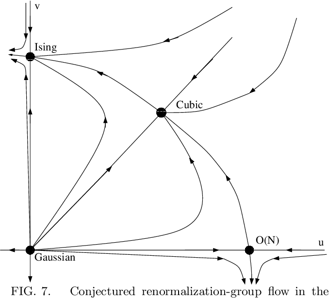
This diagram beautifully illustrates our discussion. The line labeled u=v corresponds to the pure O(n) model we analyzed. The "O(N)" point on this line is the Wilson-Fisher fixed point whose location depends on $n$. The "Ising" point is simply the special case $n=1$. The flow lines show how systems with different microscopic parameters are all drawn into the same universal critical behavior governed by one of these stable fixed points.

Conclusion

In this lesson, we have significantly broadened the scope of our investigation by generalizing from a scalar theory to the O(n) vector model. This allows us to describe a much richer set of physical systems, such as XY and Heisenberg magnets, and superfluids.

Key Takeaways:

• The O(n) model describes systems with an n-component vector order parameter where the Hamiltonian is invariant under O(n) rotations.
• The symmetry of the order parameter is a crucial ingredient in determining a system's universality class, with $n=1$, $n=2$, and $n=3$ corresponding to the Ising, XY, and Heisenberg classes, respectively.
• For systems with a continuous symmetry ($n\ge 2$), spontaneous symmetry breaking in the ordered phase gives rise to massless Goldstone modes corresponding to low-energy rotations of the order parameter.
• The RG analysis of the O(n) model yields beta functions and a Wilson-Fisher fixed point whose locations depend on both the dimension $d$ and the symmetry parameter $n$. This provides a formal basis for why critical exponents are universal for a given $(d,n)$.

Preview of the Next Lesson:

The appearance of massless Goldstone modes for $n\ge 2$ has dramatic consequences in low dimensions. These "soft" fluctuations can be so powerful that they completely destroy long-range order. In our next lesson, we will begin our study of advanced topics by proving a famous and powerful result: the Mermin-Wagner theorem, which states that a continuous symmetry cannot be spontaneously broken at any finite temperature in dimensions $d\le 2$.