Parallelizing Attention for Long-Range Dependencies

Introduction

In our previous lesson, we established the mathematical and computational framework for scaled dot-product attention. We defined it as a general-purpose mechanism, $\text{Attention}(Q,K,V)$, that functions like a differentiable, soft dictionary lookup. It computes a weighted sum of Value vectors based on the similarity between a Query vector and a set of Key vectors. So far, we've treated Q, K, and V as abstract inputs.

This lesson addresses a pivotal question: what happens when the queries, keys, and values are all derived from the same source sequence? This is the core concept of self-attention. We will derive this mechanism from first principles and explore how it revolutionizes sequence processing. Specifically, you will see how self-attention directly addresses the fundamental limitations of recurrent models, enabling the capture of complex, long-range dependencies across an entire sequence in a massively parallel fashion—a crucial feature for the high-performance systems that interest you.

Why Self-Attention? The Limits of Recurrence

Before deriving the mechanism, it's essential to understand the problems it was designed to solve. Recurrent Neural Networks (RNNs), including LSTMs and GRUs, were the dominant paradigm for sequence modeling. However, their architecture imposes two major constraints.

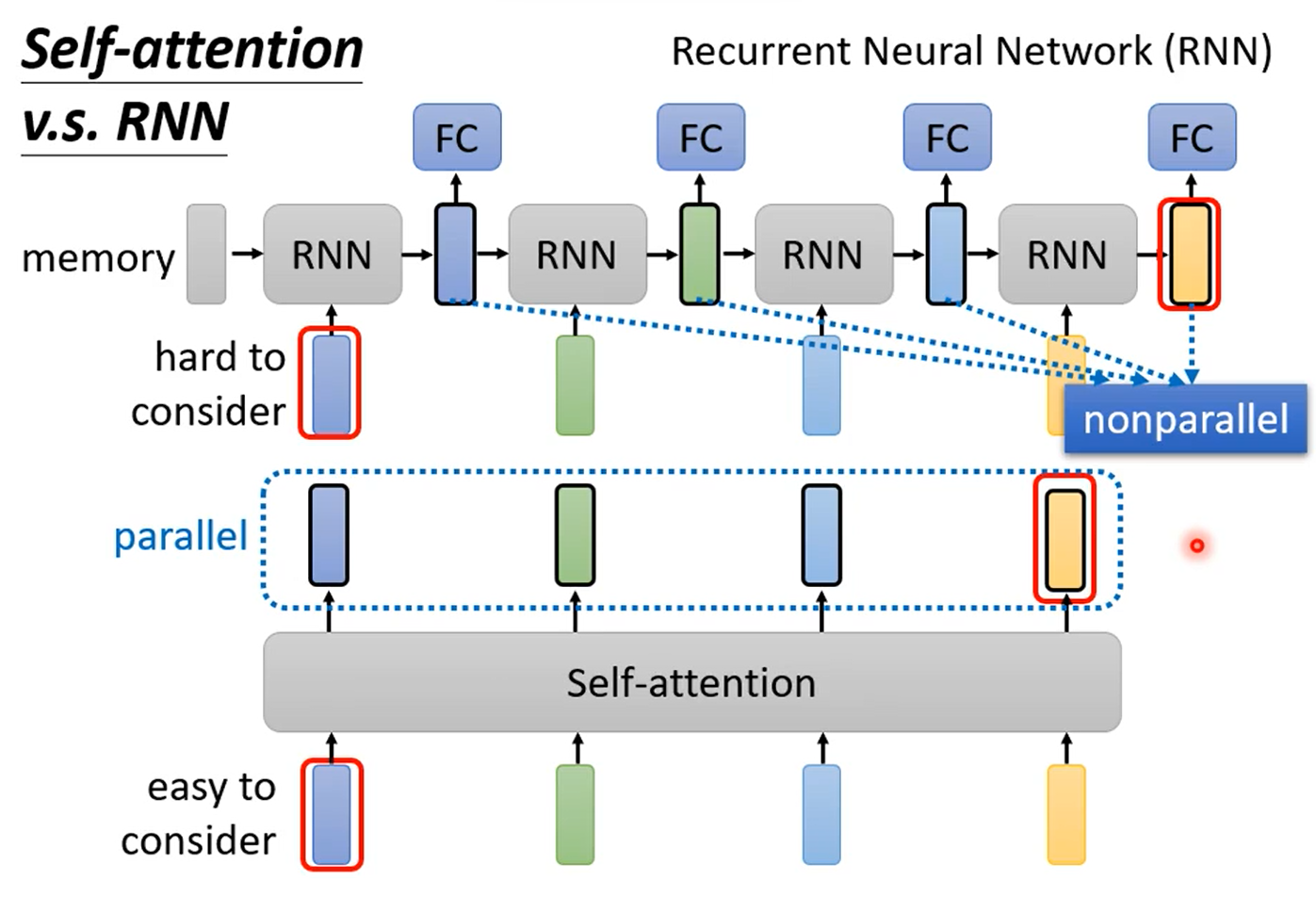
First, RNNs are inherently sequential. To compute the hidden state at timestep $t$, you must have already computed the state at $t-1$. This dependency prevents parallelization across the sequence length, creating a significant computational bottleneck.

Second, information has to travel linearly through the sequence. For two words at opposite ends of a long sentence to interact, their information must pass through every intermediate step. This long path makes it difficult for the model to learn long-range dependencies and can lead to the attenuation of gradient signals.

Let's watch a segment from a Stanford lecture that clearly articulates these two core issues.

Self-attention proposes a radical alternative: what if every word could interact directly with every other word in the sequence in a single step?

Deriving Self-Attention from First Principles

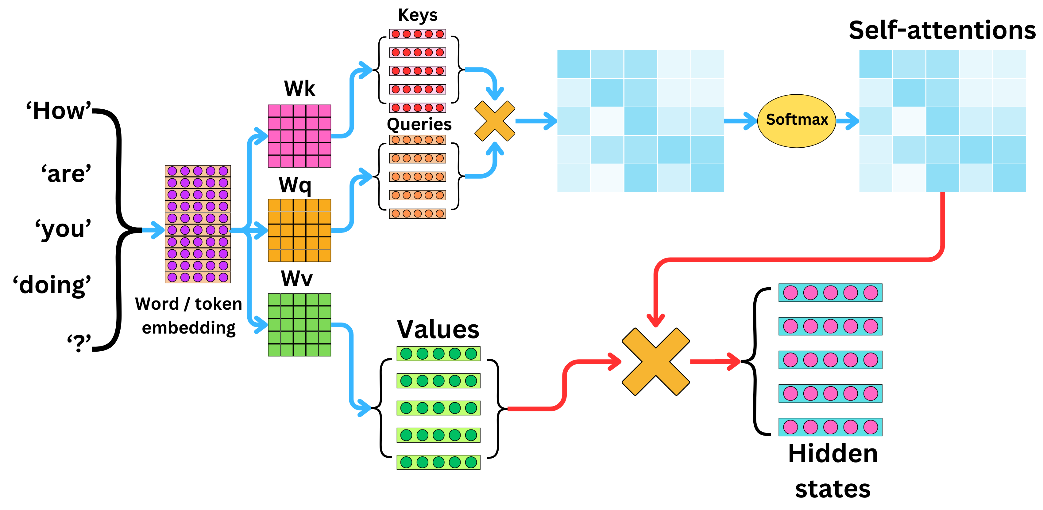
Let's build the self-attention mechanism from the ground up. We start with a sequence of $n$ input token embeddings, which we stack into a matrix $X\in {\mathbb{R}}^{n\times d_{\text{model}}}$.

In self-attention, this single input matrix $X$ is the source for our queries, keys, and values. We don't use $X$ directly; instead, we create three distinct linear projections of it by using three unique, learnable weight matrices:

• A query weight matrix: $W_Q\in {\mathbb{R}}^{d_{\text{model}}\times d_k}$
• A key weight matrix: $W_K\in {\mathbb{R}}^{d_{\text{model}}\times d_k}$
• A value weight matrix: $W_V\in {\mathbb{R}}^{d_{\text{model}}\times d_v}$

For simplicity, it's common to set the key and value dimensions to be equal, $d_k=d_v$.

The Query, Key, and Value matrices for the entire sequence are then computed as:

$$Q=X{W}_Q(Q\in {\mathbb{R}}^{n\times d_k})$$ $$K=X{W}_K(K\in {\mathbb{R}}^{n\times d_k})$$ $$V=X{W}_V(V\in {\mathbb{R}}^{n\times d_v})$$

Socratic Question: Why do we need these three separate projection matrices? What would be the limitation if we simply used the input embeddings $X$ for all three roles (i.e., $Q=K=V=X$)?

Answer

The projection matrices $W_Q, W_K, W_V$ allow the model to project the input embeddings into three different, more specialized subspaces. This gives the model flexibility. A token's role as a "query" (what information it's looking for) might be very different from its role as a "key" (what information it's signaling it has) or its "value" (the actual content it should provide). For instance, in the sentence "The robot picked up the ball, because **it** was red," the pronoun "it" might *query* for nouns in its context. Its *key* might represent that it is a pronoun looking for an antecedent. Its *value* would be the actual embedding of "it." The separate projections allow each token to learn to play these three distinct roles effectively.

With $Q$, $K$, and $V$ defined, we can now substitute them into the scaled dot-product attention formula we derived in the previous lesson. This gives us the complete equation for a self-attention layer:

$$\text{SelfAttention}(X)=\text{softmax}\left(\frac{Q{K}^T}{\sqrt{d_k}}\right)V=\text{softmax}\left(\frac{(X{W}_Q)(X{W}_K{)}^T}{\sqrt{d_k}}\right)(X{W}_V)$$

The output of this operation is a new matrix $Y\in {\mathbb{R}}^{n\times d_v}$, where each row is a new, contextually-rich representation of the corresponding input token. Each output vector is a weighted sum of all value vectors in the sequence, where the weights are determined by how well that token's query matches every other token's key.

The following diagram provides an excellent visualization of this entire process.

To solidify your understanding of this mathematical flow, the following reading from the Stanford CS224n course notes provides a concise and formal derivation.

Capturing Dependencies in Parallel

Now we can see precisely how self-attention achieves its two main goals.

1. Constant Path Length for Long-Range Dependencies:
The core of the interaction happens in the matrix multiplication $Q{K}^T$. This operation computes an $n\times n$ score matrix, where the element at position $(i,j)$ is the dot product of the query for token $i$ and the key for token $j$. This is a direct connection between token $i$ and token $j$, regardless of how far apart they are in the sequence. The path length between any two tokens is $O(1)$. This allows gradients to flow directly between distant tokens, making it vastly easier to learn long-range dependencies compared to the $O(n)$ path length in an RNN.

2. Parallel Computation:
The entire self-attention formula consists of a series of matrix multiplications. There are no sequential loops or dependencies across the time/sequence dimension ($n$). The computation for all $n$ tokens can be executed simultaneously on a GPU. This is in stark contrast to an RNN, where the computation for token $t$ must wait for token $t-1$. This massive parallelizability is a primary reason for the success and scalability of Transformer models.

The table below, from a comprehensive survey on attention, summarizes these critical differences.

The Missing Piece: Positional Information

As derived, our self-attention mechanism has a significant flaw: it is permutation equivariant. This means if you shuffle the order of the words in the input sequence, the output will be a correspondingly shuffled set of the same vectors. The model has no inherent sense of word order; it treats the input as an unordered "bag" of vectors. This is because the score ${\mathbf{q}}_i^T{\mathbf{k}}_j$ depends only on the tokens $i$ and $j$, not their positions.

To solve this, we must explicitly inject information about the position of each token into the model. This is done using positional encodings. The idea is to create a vector for each position (1, 2, 3, ...) and add it to the corresponding token embedding before it's fed into the self-attention layer.

$$X_{\text{final}}=X_{\text{embeddings}}+P_{\text{encodings}}$$

There are two common approaches:

• Sinusoidal Positional Encodings: Using a fixed set of sine and cosine functions of different frequencies to create unique positional vectors.
• Learned Positional Encodings: Creating a simple embedding layer (a lookup table) where each position index has a learnable vector.

This added positional information allows the self-attention mechanism to differentiate between "The dog chased the cat" and "The cat chased the dog."

Conclusion

In this lesson, you've derived the self-attention mechanism from first principles, understanding it as a specific and powerful application of the general attention framework from our previous session. We've seen how it directly addresses the shortcomings of recurrent models by enabling parallel computation and providing constant-time access between any two tokens in a sequence.

Key Takeaways:

• Self-Attention Derivation: Queries, Keys, and Values ($Q,K,V$) are all generated from the same input sequence $X$ via three distinct, learnable linear projections ($W_Q,W_K,W_V$).
• Parallel Dependency Capture: Self-attention computes a relevance score between every pair of tokens in a single matrix operation ($Q{K}^T$), allowing for massive parallelization and creating a direct $O(1)$ path for modeling long-range dependencies.
• Computational Advantage: Unlike the $O(n)$ sequential operations in RNNs, self-attention's complexity is dominated by matrix multiplications ($O(n^{2}d)$), which is highly efficient on modern accelerators for sequences where $n$ is smaller than the model's feature dimension $d$.
• Positional Encodings are Essential: Because the self-attention operation itself is permutation equivariant, explicit positional information must be added to the input embeddings to give the model a sense of sequence order.

Preview of the Next Lesson:

A single self-attention mechanism learns one way for tokens to interact. But what if there are multiple types of relationships we want to capture simultaneously? For example, one set of attention weights might capture syntactic dependencies, while another captures semantic similarity. In our next lesson, we will explore multi-head attention, an elegant and computationally efficient way to run multiple self-attention operations in parallel, allowing the model to jointly attend to information from different representation subspaces at different positions.