Linearizing Coordinate Transformations with Jacobians

Welcome back. Last time, you differentiated a scalar field: its gradient described how one output changes as you move in space. A coordinate transformation has several outputs, so we need a way to track how every output responds to every input direction.

That tool is the Jacobian matrix. In this lesson, you will use it to replace a nonlinear transformation with a local linear approximation, first in a picture and then for a small deformation of 3D points. Allow about 40 minutes for the video, worked examples, and PyTorch check.

A transformation seen up close

Consider a transformation $\Phi :{\mathbb{R}}^n\to {\mathbb{R}}^m$. It sends an input point $\mathbf{p}$ to an output point $\Phi (\mathbf{p})$. If you move the input by a small displacement $\mathbf{\delta }$, how far—and in which direction—does the output move?

For a differentiable transformation, the answer near $\mathbf{p}$ is

The matrix $J_{\Phi }(\mathbf{p})$ is the Jacobian at $\mathbf{p}$. It acts on displacements, not directly on absolute point positions. The term $\Phi (\mathbf{p})$ places the linear approximation at the correct output point.

The following image makes the displacement viewpoint concrete. A rectangle in input coordinates becomes a region with curved boundaries. Close to its lower-left corner, however, the two short sides are approximated by two straight output displacements.

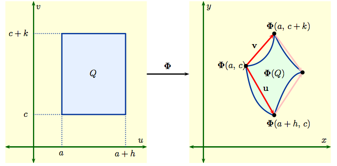
Write $\Phi (u,v)=({\Phi }_1(u,v),{\Phi }_2(u,v))$, and focus on the input corner $\mathbf{p}=(a,c)$. With column-vector coordinates, its Jacobian is

A small step $(h,0)$ produces approximately $h$ times the first column. A small step $(0,k)$ produces approximately $k$ times the second column. A step in any other direction is a combination of those two effects. Unlike a single matrix applied everywhere, this Jacobian generally changes as you move to another input point.

The connection to the previous lesson is precise: for a scalar field $f:{\mathbb{R}}^3\to \mathbb{R}$, its Jacobian is a $1\times 3$ row containing the same partial derivatives that you wrote as the column vector $\nabla f$. For a transformation with three outputs, there is one such row per output.

Linearize a nonlinear coordinate map

Take this two-dimensional transformation:

It is nonlinear, so no single matrix describes it exactly across the entire plane. Its Jacobian is

At $\mathbf{p}=(1,1)$, the input point maps to $\Phi (\mathbf{p})=(2,1.5)$, and the local matrix is

Now move by $\mathbf{\delta }=(0.1,0.05)$. Multiplication by the Jacobian predicts the change in output:

Adding that change to the output at the base point gives the linearized prediction

Direct substitution gives $\Phi (1.1,1.05)=(2.2025,1.655)$. The prediction is close, but not exact: it misses by $(0.0025,0.005)$. Those differences come from terms that depend quadratically on the displacement.

This illustrates what “local” means. Differentiability at $\mathbf{p}$ guarantees that the approximation error becomes small relative to the displacement as the displacement approaches zero:

It does not promise that a step of arbitrary size will be well approximated. Nor should you evaluate the Jacobian at the displaced point if your intention is to linearize around $\mathbf{p}$.

Check a local deformation of 3D points

The same calculation applies to 3D coordinates. Suppose a deformation acts on each point of a point cloud by

Here the first and third output coordinates depend nonlinearly on the input. Differentiating each output with respect to $x$, $y$, and $z$ gives

At $\mathbf{p}=(1,2,0)$, this becomes

For example, its first column says that a small movement in the input $x$-direction changes both the output $x$- and $z$-coordinates. Given your linear algebra preparation, you can think of the three columns as the locally transformed coordinate-direction vectors.

The following code checks the matrix with PyTorch and compares its prediction with the actual transformed point. Run it as a single block:

import torch

def deform(point):
    x, y, z = point.unbind()
    return torch.stack((
        x + 0.1 * y**2,
        y,
        z + 0.2 * x * y,
    ))

p = torch.tensor([1.0, 2.0, 0.0], dtype=torch.float64)
delta = torch.tensor([0.05, -0.10, 0.02], dtype=torch.float64)

J = torch.autograd.functional.jacobian(deform, p)
expected_J = torch.tensor(
    [[1.0, 0.4, 0.0],
     [0.0, 1.0, 0.0],
     [0.4, 0.2, 1.0]],
    dtype=torch.float64,
)
torch.testing.assert_close(J, expected_J)

predicted = deform(p) + J @ delta
actual = deform(p + delta)
error = actual - predicted

print("Jacobian:\n", J)
print("linearized output:", predicted)
print("actual output:    ", actual)
print("approximation error:", error)

half_delta = delta / 2
half_error = deform(p + half_delta) - (
    deform(p) + J @ half_delta
)
print("error with half-sized step:", half_error)
torch.testing.assert_close(half_error, error / 4)

The predicted output is $(1.410,1.900,0.420)$; the actual output is $(1.411,1.900,0.419)$. In this particular deformation, halving the step quarters the error because the terms omitted by the linear approximation are quadratic in the displacement. That exact quartering is a feature of this example, not a rule to assume for every transformation.

Notice the difference from checking a scalar gradient. deform(p) has three outputs, and J has shape (3, 3): it retains the response of each output to each input coordinate. A gradient of a sum of those outputs would combine the rows and lose that separate information.

For a point cloud, you can repeat this local calculation at different points. The deformation rule stays the same, but $J_{\Psi }(\mathbf{p})$ varies with $\mathbf{p}$, so nearby parts of the cloud can undergo different local stretches and shears. That is why one global matrix cannot generally replace a nonlinear geometric transformation.

Takeaways

A Jacobian turns a small input displacement into a first-order prediction of the output displacement. Its rows correspond to output components, its columns correspond to input directions, and it must be evaluated at the point around which you are linearizing. The full local prediction includes the transformed base point: $\Phi (\mathbf{p})+J_{\Phi }(\mathbf{p})\mathbf{\delta }$.

Next, you will use this same derivative-matrix viewpoint in reverse: deriving how gradients pass backward through an affine layer and a ReLU activation.