Phonon-Limited Resistivity: High and Low Temperature Limits

Hello! Welcome to our lesson on phonon-limited resistivity.

In our previous session, we used Fermi's Golden Rule to find the microscopic scattering rate, $1/\tau$, for an electron interacting with phonons. We even saw a sneak peek in a mini-exercise: in the high-temperature limit, the acoustic phonon scattering rate is proportional to temperature, $1/\tau \propto T$, which suggests that resistivity $\rho \propto T$.

Today, we will formalize this connection. Our goal is to derive the full temperature dependence of phonon-limited resistivity, from the famous linear behavior at high temperatures to the characteristic power law at low temperatures. To bridge the gap between microscopic scattering and macroscopic transport, we'll use a powerful semi-classical tool: the Boltzmann Transport Equation (BTE). This will lead us to the celebrated Bloch-Grüneisen formula.

1. The Boltzmann Transport Equation and the Relaxation Time Approximation

To understand how a collection of electrons responds to an electric field, we need to track their distribution in phase space. The distribution function, $f(\mathbf{r},\mathbf{k},t)$, tells us the probability of finding an electron at position $\mathbf{r}$ with crystal momentum $\mathbf{k}$ at time $t$. The BTE is essentially a continuity equation that describes how this function evolves. It states that the total time derivative of $f$ is the sum of changes due to external fields (drift) and scattering events (collisions):

$$\frac{df}{dt}={\left(\frac{\partial f}{\partial t}\right)}_{\text{drift}}+{\left(\frac{\partial f}{\partial t}\right)}_{\text{coll}}$$

The collision term is notoriously complex, as it involves an integral over all possible scattering processes. To make progress, we introduce the Relaxation Time Approximation (RTA). This approximation assumes that any deviation from the equilibrium distribution, $f_0$ (the Fermi-Dirac distribution), decays exponentially back to equilibrium with a characteristic time $\tau$.

$${\left(\frac{\partial f}{\partial t}\right)}_{\text{coll}}=-\frac{f-f_0}{\tau }$$

This $\tau$ is the average time between collisions that randomize the electron's momentum, and it is directly related to the scattering rates we calculated in the last lesson.

To see how the BTE is set up and how the RTA is applied, please review the first part of the following resource.

2. Deriving the Electrical Conductivity

With the BTE and RTA in hand, we can now calculate the electrical conductivity, $\sigma$. Let's consider a simple, steady-state ($\frac{df}{dt}=0$) and spatially uniform system, where the only external force is from a constant electric field, $\mathbf{E}$. The BTE becomes:

$${\left(\frac{\partial f}{\partial t}\right)}_{\text{drift}}+{\left(\frac{\partial f}{\partial t}\right)}_{\text{coll}}=0$$

The drift term for an electron with charge $-e$ is ${\left(\frac{\partial f}{\partial t}\right)}_{\text{drift}}=-\dot{\mathbf{k}}\cdot {\nabla }_{\mathbf{k}}f=-\frac{-e\mathbf{E}}{\hslash }\cdot {\nabla }_{\mathbf{k}}f$. Assuming the field is weak, the distribution $f$ is only slightly perturbed from equilibrium, $f\approx f_0$. So, we can approximate ${\nabla }_{\mathbf{k}}f\approx {\nabla }_{\mathbf{k}}{f}_0$. Using the chain rule, ${\nabla }_{\mathbf{k}}{f}_0=\frac{\partial f_0}{\partial ϵ}{\nabla }_{\mathbf{k}}ϵ=\frac{\partial f_0}{\partial ϵ}\hslash {\mathbf{v}}_{\mathbf{k}}$.

Plugging this into the BTE:

$$\frac{e\mathbf{E}}{\hslash }\cdot (\hslash {\mathbf{v}}_{\mathbf{k}}\frac{\partial f_0}{\partial ϵ})-\frac{f-f_0}{\tau }=0$$

Solving for $f$, we find the non-equilibrium distribution function:

$$f(\mathbf{k})=f_0(\mathbf{k})+e\tau (\mathbf{k})({\mathbf{v}}_{\mathbf{k}}\cdot \mathbf{E})\left(-\frac{\partial f_0}{\partial ϵ}\right)$$

The term $-\frac{\partial f_0}{\partial ϵ}$ is sharply peaked at the Fermi energy, ${ϵ}_F$. This tells us that only electrons near the Fermi surface contribute to conduction, as expected.

The electrical current density $\mathbf{J}$ is the sum of velocities of all electrons. Using our new distribution $f(\mathbf{k})$:

$$\mathbf{J}=-e\int {\mathbf{v}}_{\mathbf{k}}f(\mathbf{k})\frac{2d^{3}k}{(2\pi {)}^3}=-e\int {\mathbf{v}}_{\mathbf{k}}\left[f_0(\mathbf{k})+e\tau (\mathbf{k})({\mathbf{v}}_{\mathbf{k}}\cdot \mathbf{E})\left(-\frac{\partial f_0}{\partial ϵ}\right)\right]\frac{2d^{3}k}{(2\pi {)}^3}$$

The integral of ${\mathbf{v}}_{\mathbf{k}}{f}_0(\mathbf{k})$ is zero due to symmetry (for every electron with velocity $\mathbf{v}$, there's one with $-\mathbf{v}$ in equilibrium). We are left with the contribution from the perturbation. For an isotropic system where $\tau$ only depends on energy, this simplifies to the familiar Drude-like formula $\mathbf{J}=\sigma \mathbf{E}$, where the resistivity is $\rho =1/\sigma =\frac{m^{\ast }}{n{e}^2{\tau }_F}$, with ${\tau }_F$ being the relaxation time for electrons at the Fermi surface.

3. The Role of Umklapp Scattering

Before deriving the temperature dependence, we must address a crucial subtlety. Not all scattering events are equally effective at creating resistance. Small-angle scattering events barely change an electron's forward momentum and thus do little to degrade an electrical current. Large-angle scattering, especially back-scattering, is what truly causes resistance.

Electron-phonon scattering must conserve both energy and crystal momentum. Crystal momentum conservation is ${\mathbf{k}}^{\prime }=\mathbf{k}+\mathbf{q}+\mathbf{G}$, where $\mathbf{G}$ is a reciprocal lattice vector.

• Normal Processes ($\mathbf{G}=0$): Crystal momentum is conserved. At low temperatures, only low-$q$ phonons are available, leading to only small-angle scattering.
• Umklapp Processes ($\mathbf{G}\ne 0$): Crystal momentum is not conserved. An electron can be scattered across the Brillouin zone, effectively reversing its direction. This is a very efficient mechanism for resistance.

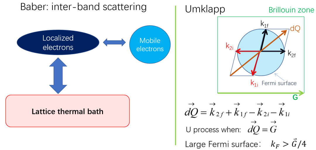
Umklapp processes require phonons with sufficient momentum to bridge the gap to another Brillouin zone, i.e., $q\sim G/2$. This is why they are suppressed at very low temperatures but become dominant as $T$ increases.

4. Deriving the Temperature Dependence of Resistivity

We are now ready to combine our understanding of the relaxation time $\tau$ and the conductivity formula to find $\rho (T)$. The calculation involves integrating the scattering probability over all possible final states, weighted by a factor of $(1-\cos \theta )$ that accounts for the ineffectiveness of forward scattering. This leads to the Bloch-Grüneisen Law.

Let's study the derivation for the two key temperature limits.

Let's summarize the key physical arguments from that derivation.

High-Temperature Limit ($T\gg {\Theta }_D$)

• Physics: The thermal energy $k_{B}T$ is much larger than the maximum phonon energy $k_B{\Theta }_D$. All phonon modes are excited, and their occupation number follows the classical equipartition theorem: $n_q\approx \frac{k_{B}T}{\hslash {\omega }_q}\gg 1$.
• Scattering: Electrons can scatter by large angles, as phonons with large momentum $q$ (up to $2k_F$) are abundant. Umklapp scattering is very active.
• Derivation: The scattering rate $1/\tau$ is proportional to the number of phonons, $n_q$. Since $n_q\propto T$, the scattering rate is also proportional to temperature.
• Result: $\rho \propto \frac{1}{\tau }\propto T$. This gives the classic linear dependence of resistivity observed in metals at and above room temperature.

Low-Temperature Limit ($T\ll {\Theta }_D$)

• Physics: Thermal energy is low. Only low-energy, long-wavelength acoustic phonons with $\hslash {\omega }_q\sim k_{B}T$ are available. The maximum phonon wavevector is small, $q_{max}\sim T/{\Theta }_D\cdot k_F\ll k_F$.
• Scattering: Umklapp processes are exponentially suppressed because there are no phonons with enough momentum. Scattering is restricted to small angles, $\theta \approx q/k_F\propto T$.
• Derivation: This case is more subtle. The resistivity depends on a product of factors:
  1. Scattering probability: Proportional to $n_q$, which for $\hslash {\omega }_q\sim k_{B}T$ is roughly constant, but the number of available phonons to scatter with goes as $q_{max}^3\propto T^3$.
  2. Scattering inefficiency: Each small-angle scattering event is inefficient at causing resistance. The effectiveness goes as $(1-\cos \theta )\approx {\theta }^2/2\propto (q/k_F{)}^2\propto T^2$.
• Result: Combining these effects, the resistivity scales as $\rho \propto T^3\times T^2=T^5$.

This $\rho \propto T^5$ dependence is a hallmark of electron-phonon scattering in 3D metals at very low temperatures.

5. The Full Bloch-Grüneisen Formula and Experimental Reality

The high-T and low-T behaviors are limits of a more general integral expression. A recent research paper provides a very clean, modern presentation of this formula and its implications.

The general BG formula for 3D ($n=5$) is:

$$\rho (T)\propto T^5{\int }_0^{{\Theta }_D/T}\frac{z^5}{(e^z-1)(1-e^{-z})}dz$$

This integral correctly reproduces the $T^5$ and $T$ limits. As you saw in the paper, this can be written elegantly in dimensionless variables. The analysis in that paper highlights a fascinating point relevant to your experimental work: in the intermediate temperature range ($T\sim {\Theta }_D/5$ to $T\sim {\Theta }_D$), the resistivity curve looks linear but does not extrapolate to the correct residual resistivity at $T=0$.

Test your understanding!

An experimentalist measures the resistivity of a very pure copper sample (${\Theta }_D\approx 343$ K) between 77 K and 300 K. They find the data is almost perfectly linear. They perform a linear fit to this data and extrapolate it to $T=0$ K to determine the residual resistivity ${\rho }_0$. Based on the discussion in the Das Sarma paper, will their extrapolated value for ${\rho }_0$ likely be an overestimate, an underestimate, or an accurate measure of the true residual resistivity? Why?

Show answer

The extrapolated value will likely be an underestimate of the true residual resistivity. In some cases, it might even be negative.

The reason, as shown in the paper (e.g., Fig. 1), is that in this intermediate temperature range ($T/{\Theta }_D$ is roughly 0.2 to 0.9), the BG resistivity curve is slightly concave up. A straight line tangent to this curve will have a negative y-intercept. When adding the true residual resistivity ${\rho }_0$, the total resistivity is $\rho (T)={\rho }_0+{\rho }_{phonon}(T)$. Extrapolating the linear-looking part of this total curve will yield an intercept of ${\rho }_0+A$, where $A$ is the negative intercept of the phonon part. Since $A<0$, the extrapolated value ${\rho }_0+A$ is less than the true value ${\rho }_0$.

Conclusion

Today we have built a solid bridge from the quantum mechanical scattering rates to the macroscopic, temperature-dependent electrical resistivity of a metal.

Key Takeaways:

• The Boltzmann Transport Equation in the Relaxation Time Approximation provides the theoretical framework to calculate conductivity from microscopic scattering.
• Resistivity is caused by scattering events that change the direction of electron momentum. Umklapp processes are particularly effective at this.
• The Bloch-Grüneisen law describes the temperature dependence of phonon-limited resistivity:
  • At high temperatures ($T\gg {\Theta }_D$), resistivity is linear in temperature: $\rho \propto T$.
  • At low temperatures ($T\ll {\Theta }_D$), resistivity falls off sharply: $\rho \propto T^5$.
• Extracting material parameters like residual resistivity from experimental data requires care, as simple linear extrapolations from intermediate temperatures can be misleading.

Preview of the Next Lesson

We have treated the electron and phonon systems as distinct entities that interact. However, a strong interaction can fundamentally alter the electron itself. When an electron moves through a polar crystal, it drags a cloud of lattice distortion (phonons) with it. This composite object is no longer a bare electron but a new quasiparticle called a polaron. In our next lesson, we will explore the formation of polarons and calculate how the electron-phonon interaction renormalizes the electron's effective mass.