Heat Sharing in Parallel Thermal-Resistance Networks

Hello! Last lesson, you estimated a junction temperature by adding resistances along a path that carried the same heat rate through every segment. A PCB-mounted component seldom has only one route for its heat: some can leave through the package top, while some enters the board. Today you will calculate how the component’s power divides between such routes, then reconnect them to the shared enclosure-to-ambient path. This gives you a more useful hand-calculation benchmark for a later Fluent model.

What makes two thermal paths parallel?

Two resistances are in parallel when they connect the same pair of temperature nodes. They therefore experience the same temperature difference, but they generally carry different heat rates. At a node where a component releases $P$ watts, steady-state energy conservation requires the branch rates to sum to $P$.

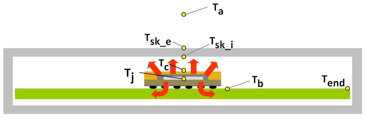
The physical sketch below shows why a PCB component invites this kind of model. Heat can travel upward from the package and downward into the board. The labels mark possible temperature locations, not necessarily surfaces that are each uniform in temperature.

Kody Powell’s Heat Transfer - Chapter 3 - Thermal Resistances in Parallel, Contact Resistance, R-Value develops the governing rule using side-by-side wall paths, then shows how each branch can itself contain series resistances. Watch the selected portions for the node structure rather than for the wall geometry; the same calculation will apply to our component.

Suppose a junction at $T_j$ sends heat through two complete routes that both end at a surface at $T_w$. Call their total resistances $R_{\mathrm{top}}$ and $R_{\mathrm{board}}$. Each route sees the same drop $T_j-T_w$, so

Combining those statements gives the equivalent parallel resistance:

For two branches, the equivalent can also be written

Do not add the two branch resistances as though all $P$ watts passed through both. Their temperature drops are equal; their heat rates are not. The lower-resistance route carries more heat. Equivalently, heat divides in proportion to branch conductance, $1/R$:

These expressions use $K/W$ for resistance and watts for power. As a quick physical check, adding a functioning parallel route must make the equivalent resistance lower than either individual route.

Identify complete branches before calculating

A package-top route and a board route can each include several series elements. For example, a top branch might include junction-to-top conduction followed by transfer across the enclosed space to the wall. A board branch might include junction-to-board conduction followed by transfer from the board toward the wall. Add the elements inside each route first, provided the same branch heat rate crosses those elements.

Texas Instruments’ AN-2020 Thermal Design By Insight, Not Hindsight, Section 2, “Definitions Description of Thermal Terms,” describes a junction-to-ambient resistance as the combined effect of multiple heat paths. Its Figure 2 supplies a package-top and exposed-pad/PCB example. Read it as an example of network topology, not as a ready-made resistance value for a sealed enclosure.

The next network drawing makes the split explicit. At $T_J$, the source $P$ divides into a top route and a board route; each route has its own intermediate temperatures and heat rate.

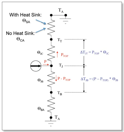
There is an important adaptation for your sealed-enclosure study. In the drawing, a branch appears to reach ambient directly after leaving the package or board. Inside a sealed enclosure, neither the internal air nor an internal heat sink is the external ambient. A branch resistance must include the remaining transfer to its stated endpoint—perhaps an enclosure-wall temperature—before it can be placed in parallel with another branch ending there. Any wall-to-external-ambient resistance shared by the routes belongs after their recombination, not separately in both branches.

Calculate the split, then the shared temperature rise

Return to the earlier illustrative enclosure: three components dissipate $3\mathrm{W}$, $2\mathrm{W}$, and $1\mathrm{W}$. The exterior surface was estimated at $35^{\circ }\mathrm{C}$ with external ambient at $25^{\circ }\mathrm{C}$. We will use that exterior temperature as an assumed common endpoint for two routes from the $3\mathrm{W}$ component. The following branch values are illustrative model inputs, not measured package specifications:

Here $w$ denotes the modeled exterior-wall endpoint. Each second segment is an effective resistance all the way to that endpoint; it must include the transfers that the simplified path leaves implicit.

First combine the routes:

The junction rise above the assumed $35^{\circ }\mathrm{C}$ wall temperature is therefore $3(2)=6^{\circ }\mathrm{C}$, giving $T_j=41^{\circ }\mathrm{C}$. Both complete branches have a $6^{\circ }\mathrm{C}$ drop, so their rates are

They sum to the specified $3\mathrm{W}$. Notice that “board carries twice as much heat” does not mean the board branch has twice the temperature drop. Its resistance is half as large, so it carries twice the rate under the same drop.

You can also recover intermediate node temperatures using each branch’s own rate. The top-case drop from the junction is $1\mathrm{W}\times 1K/W=1^{\circ }\mathrm{C}$, giving $40^{\circ }\mathrm{C}$. The board-node drop is $2\mathrm{W}\times 1K/W=2^{\circ }\mathrm{C}$, giving $39^{\circ }\mathrm{C}$. The two intermediate nodes need not have the same temperature: only the endpoints used to define the parallel branches must match.

Finally, check the shared downstream path. The enclosure exterior rejects all $6\mathrm{W}$ generated by the three components. Its $10^{\circ }\mathrm{C}$ rise above ambient corresponds to an effective exterior-to-ambient resistance of

That resistance carries $6\mathrm{W}$, not merely the $1\mathrm{W}$ or $2\mathrm{W}$ from either branch of our selected component. The other components’ heat has joined the enclosure’s total load. This is why calculating the branch split and calculating the enclosure’s ambient rise are related but distinct tasks.

Where the simple network stops being reliable

Parallel reduction depends on the endpoints being defensible common-temperature nodes. A compact PCB model might assign one board temperature to a wide region, yet the real board can have strong temperature gradients. Likewise, heat reaching different places on an enclosure wall may encounter different local wall temperatures. Calling those places a single node is an approximation, not a consequence of drawing them together.

Watch the final selected part of Powell’s lesson for this distinction between the thermal-circuit representation and a spatial temperature field.

There are two further cautions for the sealed enclosure. First, effective resistances involving internal convection or radiation can change as temperatures change; a fixed-resistance split is then an estimate for the stated operating conditions. Second, a published junction-to-ambient resistance is already a whole-network result for particular test conditions. It is not an extra resistor to place in series with both of your newly defined branches.

The network remains valuable because its assumptions are inspectable. When you later build the Fluent model, temperatures at the junction representation, package top, board, and enclosure can be compared with the corresponding network nodes. Heat-transfer rates through selected surfaces can also test the predicted $1\mathrm{W}$/$2\mathrm{W}$ split—provided the surfaces actually separate those routes without counting the same heat twice.

Closing perspective

For parallel thermal paths, use a common temperature drop across complete branches, calculate each branch rate from its own resistance, and check that the rates sum to the source power. Combine series elements within a branch before taking the parallel equivalent. Once branches rejoin, any shared downstream resistance carries the combined heat rate—and, in a multi-component enclosure, may carry heat from other sources too.

Next, you will return to the steady-state energy balance for the sealed enclosure, using it to account systematically for heat generated inside and heat rejected at its boundaries.