Quasiparticle Properties from Self-Energy

Hello! In our last lesson, we derived the Dyson equation, G^{-1} = G_0^{-1} - \Sigma, which provides a powerful framework for understanding how interactions modify the behavior of electrons in a solid. We saw that the full Green's function takes the form G(\mathbf{k}, \omega) = [\omega - \epsilon^0_{\mathbf{k}} - \Sigma(\mathbf{k}, \omega)]^{-1}, hinting that the self-energy \Sigma is responsible for renormalizing the particle's properties.

Today, we will make this connection explicit. Our goal is to extract quasiparticle energies and lifetimes from the real and imaginary parts of the self-energy. We will formalize the procedure for finding the properties of the "dressed" particles, or quasiparticles, which are the true elementary excitations of an interacting system. This process lies at the heart of connecting many-body theory to experimental observables.

1. The Quasiparticle Pole

The poles of the Green's function identify the energies of the system's elementary excitations. For the non-interacting Green's function, G_0(\mathbf{k}, \omega) = [\omega - \epsilon^0_{\mathbf{k}} + i\eta]^{-1}, the pole is simply at the bare particle energy \epsilon^0_{\mathbf{k}}. For the interacting Green's function G(\mathbf{k}, \omega), the poles are the complex energies \omega that satisfy the equation:

$$\omega -{ϵ}_{\mathbf{k}}^0-\Sigma (\mathbf{k},\omega )=0$$

Since the self-energy \Sigma is itself a function of \omega, solving this equation is non-trivial. The solutions will be complex numbers, \omega_p = E_{\mathbf{k}} - i\Gamma_{\mathbf{k}}, where E_{\mathbf{k}} is the quasiparticle energy and \Gamma_{\mathbf{k}} is its decay rate.

The concept of a quasiparticle is most useful when it is "well-defined," meaning its decay rate \Gamma_{\mathbf{k}} is small compared to its energy E_{\mathbf{k}}. This condition is met for excitations close to the Fermi surface, which is the central tenet of Landau's Fermi liquid theory. Assuming a well-defined quasiparticle exists, we can analyze the Green's function near the quasiparticle pole.

To understand the roles of the real and imaginary parts of the self-energy in this process, let's start with a clear definition.

2. Extracting Quasiparticle Properties: The Quasiparticle Approximation

As the notes suggest, to find the properties of a quasiparticle pole near the real axis, we can expand the self-energy around the quasiparticle energy E_{\mathbf{k}}. The quasiparticle energy E_{\mathbf{k}} itself is the real energy that satisfies:

$$E_{\mathbf{k}}={ϵ}_{\mathbf{k}}^0+\text{Re}{\Sigma }^R(\mathbf{k},E_{\mathbf{k}})$$

This is a self-consistent equation for E_{\mathbf{k}}. Now, we perform a first-order Taylor expansion of \Sigma^R(\mathbf{k}, \omega) around \omega = E_{\mathbf{k}}:

$${\Sigma }^R(\mathbf{k},\omega )\approx {\Sigma }^R(\mathbf{k},E_{\mathbf{k}})+(\omega -E_{\mathbf{k}}){\frac{\partial {\Sigma }^R(\mathbf{k},\omega )}{\partial \omega }|}_{\omega =E_{\mathbf{k}}}$$

Substituting this into the denominator of the Green's function, \omega - \epsilon^0_{\mathbf{k}} - \Sigma^R(\mathbf{k}, \omega), gives:

$$\approx \omega -{ϵ}_{\mathbf{k}}^0-\left(\text{Re}{\Sigma }^R(\mathbf{k},E_{\mathbf{k}})+i\text{Im}{\Sigma }^R(\mathbf{k},E_{\mathbf{k}})+(\omega -E_{\mathbf{k}}){\frac{\partial {\Sigma }^R}{\partial \omega }|}_{E_{\mathbf{k}}}\right)$$

Using our definition of E_{\mathbf{k}}, the \omega - \epsilon^0_{\mathbf{k}} - \text{Re}\Sigma^R(\mathbf{k}, E_{\mathbf{k}}) terms combine to \omega - E_{\mathbf{k}}. Grouping the terms, we get:

$$(\omega -E_{\mathbf{k}})\left(1-{\frac{\partial {\Sigma }^R}{\partial \omega }|}_{E_{\mathbf{k}}}\right)-i\text{Im}{\Sigma }^R(\mathbf{k},E_{\mathbf{k}})$$

Let's define the quasiparticle weight (or renormalization constant) Z_{\mathbf{k}} as:

$$Z_{\mathbf{k}}={\left(1-{\frac{\partial \text{Re}{\Sigma }^R(\mathbf{k},\omega )}{\partial \omega }|}_{\omega =E_{\mathbf{k}}}\right)}^{-1}$$

Assuming the derivative of the imaginary part is small, the denominator of G becomes Z_{\mathbf{k}}^{-1}(\omega - E_{\mathbf{k}}) - i\text{Im}\Sigma^R(\mathbf{k}, E_{\mathbf{k}}). The Green's function near the pole is then:

$$G^R(\mathbf{k},\omega )\approx \frac{1}{Z_{\mathbf{k}}^{-1}(\omega -E_{\mathbf{k}})-i\text{Im}{\Sigma }^R(\mathbf{k},E_{\mathbf{k}})}=\frac{Z_{\mathbf{k}}}{(\omega -E_{\mathbf{k}})-i{Z}_{\mathbf{k}}\text{Im}{\Sigma }^R(\mathbf{k},E_{\mathbf{k}})}$$

This is a Lorentzian (or Breit-Wigner) form, characteristic of a decaying particle. By comparing this to the general form of a propagator for a decaying state, Z/(\omega - E + i\Gamma), we can identify all the quasiparticle properties.

Summary of Quasiparticle Properties:

1. Energy E_{\mathbf{k}}: The renormalized energy, found by solving the self-consistent equation:

   $$E_{\mathbf{k}}={ϵ}_{\mathbf{k}}^0+\text{Re}{\Sigma }^R(\mathbf{k},E_{\mathbf{k}})$$

2. Lifetime \tau_{\mathbf{k}}: The lifetime is related to the decay rate \Gamma_{\mathbf{k}}. For the retarded Green's function, causality requires the pole to be in the lower half of the complex plane, which means the decay rate must be positive. This requires \text{Im}\Sigma^R(\mathbf{k}, \omega) to be negative for particle states (\omega > E_F). The decay rate is:

   $${\Gamma }_{\mathbf{k}}=-Z_{\mathbf{k}}\text{Im}{\Sigma }^R(\mathbf{k},E_{\mathbf{k}})$$

   The quasiparticle lifetime is then \tau_{\mathbf{k}} = \hbar / (2\Gamma_{\mathbf{k}}).

3. Weight Z_{\mathbf{k}}: The quasiparticle weight, defined as:

   $$Z_{\mathbf{k}}={\left(1-{\frac{\partial \text{Re}{\Sigma }^R(\mathbf{k},\omega )}{\partial \omega }|}_{\omega =E_{\mathbf{k}}}\right)}^{-1}$$

   Z_{\mathbf{k}} represents the overlap between the "bare" single-particle state and the true, dressed quasiparticle state. In interacting systems, 0 < Z_{\mathbf{k}} \le 1. A smaller Z_{\mathbf{k}} indicates stronger correlation effects, as the quasiparticle is a more complex mixture of many-body configurations.

These definitions provide a complete recipe for calculating quasiparticle properties once the self-energy is known.

3. Behavior Near the Fermi Surface

The framework we've developed is central to Landau's Fermi liquid theory. A defining feature of a Fermi liquid is that quasiparticles near the Fermi surface are long-lived. The scattering rate must vanish as a quasiparticle's energy approaches the Fermi energy, E_F.

Microscopic calculations show that for a 3D electron gas at T=0, the imaginary part of the self-energy behaves as:

$$\text{Im}{\Sigma }^R(\mathbf{k},\omega )\propto -(\omega -E_F{)}^2$$

This quadratic dependence arises from phase space constraints: a particle trying to decay near the Fermi surface has very few available final states to scatter into that conserve both energy and momentum. Since \Gamma_{\mathbf{k}} \propto -\text{Im}\Sigma^R, the decay rate also vanishes quadratically, \Gamma_{\mathbf{k}} \propto (E_{\mathbf{k}} - E_F)^2. This confirms that quasiparticles at the Fermi surface (E_{\mathbf{k}} = E_F) have an infinite lifetime, stabilizing the Fermi liquid state. At finite temperature, a similar calculation yields a T^2 dependence for the scattering rate.

4. Experimental Connection: ARPES and the Self-Energy

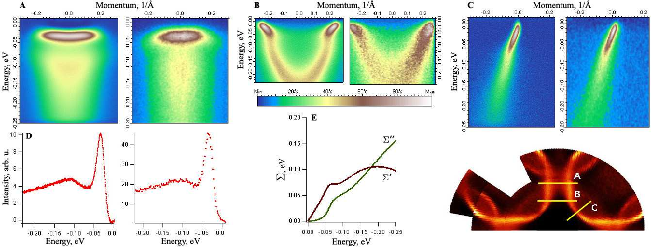
These concepts are not just theoretical constructs. Angle-Resolved Photoemission Spectroscopy (ARPES) provides a direct experimental window into the properties of quasiparticles. As we will explore more formally in a future lesson, the intensity measured in an ARPES experiment is directly proportional to the spectral function A(\mathbf{k}, \omega) = -\frac{1}{\pi}\text{Im}G^R(\mathbf{k}, \omega).

Using our approximate form for G^R, the spectral function near a quasiparticle pole is a Lorentzian:

$$A(\mathbf{k},\omega )\approx \frac{Z_{\mathbf{k}}}{\pi }\frac{{\Gamma }_{\mathbf{k}}}{(\omega -E_{\mathbf{k}}{)}^2+{\Gamma }_{\mathbf{k}}^2}$$

This shows that an ARPES experiment will observe peaks in its energy distribution curves (EDCs). By fitting these peaks, one can directly extract the experimental quasiparticle properties:

• The peak position gives the quasiparticle energy E_{\mathbf{k}}.
• The peak width (FWHM) is 2\Gamma_{\mathbf{k}}, which gives the lifetime \tau_{\mathbf{k}}.
• The integrated intensity of the peak is proportional to the quasiparticle weight Z_{\mathbf{k}}.

By performing this analysis at many momentum points \mathbf{k}, physicists can map out the full quasiparticle band structure E_{\mathbf{k}} and, by inverting the relations we've derived, extract the underlying self-energy \Sigma(\mathbf{k}, \omega).

Test your understanding!

Imagine you are analyzing a quasiparticle peak for a state with bare energy \epsilon^0_{\mathbf{k}} = 0.1 eV (relative to the Fermi energy). By fitting ARPES data, you extract a self-energy that, near the expected peak, can be approximated by \Sigma^R(\omega) = -0.5\omega - i(0.1)\omega^2. All energies are in eV.

1. Find the renormalized quasiparticle energy E_{\mathbf{k}}.
2. Calculate the quasiparticle weight Z_{\mathbf{k}}.
3. Determine the quasiparticle lifetime \tau_{\mathbf{k}} in femtoseconds. (Use \hbar \approx 6.582 \times 10^{-16} eV·s).

Show answer

1. Energy E_{\mathbf{k}}: We need to solve E_{\mathbf{k}} = \epsilon^0_{\mathbf{k}} + \text{Re}\Sigma^R(E_{\mathbf{k}}):
   E_{\mathbf{k}} = 0.1 - 0.5 E_{\mathbf{k}}
1.5 E_{\mathbf{k}} = 0.1
E_{\mathbf{k}} = 0.1 / 1.5 \approx 0.067 eV.

2. Weight Z_{\mathbf{k}}: We need the derivative of \text{Re}\Sigma^R:
   \partial(\text{Re}\Sigma^R)/\partial\omega = -0.5.
   Z_{\mathbf{k}} = (1 - (-0.5))^{-1} = 1 / 1.5 \approx 0.67.

3. Lifetime \tau_{\mathbf{k}}: First, find the decay rate \Gamma_{\mathbf{k}} = -Z_{\mathbf{k}} \text{Im}\Sigma^R(E_{\mathbf{k}}):
   \text{Im}\Sigma^R(E_{\mathbf{k}}) = -0.1 \times (0.067)^2 \approx -0.000449 eV.
   \Gamma_{\mathbf{k}} = -(0.67) \times (-0.000449) \approx 0.00030 eV.
   Now, calculate the lifetime \tau_{\mathbf{k}} = \hbar / (2\Gamma_{\mathbf{k}}):
   \tau_{\mathbf{k}} = (6.582 \times 10^{-16} \text{ eV·s}) / (2 \times 0.00030 \text{ eV}) \approx 1.097 \times 10^{-12} s.
   This is approximately 1097 femtoseconds (fs).

Conclusion

In this lesson, we have solidified the physical meaning of the self-energy. By analyzing the poles of the dressed Green's function, we have developed a precise procedure to determine the properties of quasiparticles—the emergent, dressed entities that populate the world of interacting electrons.

Key Takeaways:

• The poles of the interacting Green's function give the complex energies of quasiparticles.
• The quasiparticle energy E_{\mathbf{k}} is determined by the real part of the self-energy via the self-consistent equation E_{\mathbf{k}} = \epsilon^0_{\mathbf{k}} + \text{Re}\Sigma^R(\mathbf{k}, E_{\mathbf{k}}).
• The quasiparticle lifetime \tau_{\mathbf{k}} is determined by the imaginary part of the self-energy, with the decay rate given by \Gamma_{\mathbf{k}} = -Z_{\mathbf{k}} \text{Im}\Sigma^R(\mathbf{k}, E_{\mathbf{k}}).
• The quasiparticle weight Z_{\mathbf{k}} measures the overlap with the bare particle state and is related to the energy derivative of \text{Re}\Sigma^R.
• These theoretical quantities are directly accessible through experiments like ARPES, which measure the spectral function A(\mathbf{k}, \omega).

Preview of the Next Lesson

Having completed our deep dive into the Green's function formalism, from diagrams to quasiparticles, we will now pivot to a new, major topic in condensed matter physics: magnetism. In the next lesson, we will begin our study of magnetism in solids by answering a fundamental question: what is the quantum mechanical origin of the interaction between localized magnetic moments? We will derive the Heisenberg exchange Hamiltonian as an effective low-energy model for interacting localized spins, setting the stage for understanding phenomena like ferromagnetism and antiferromagnetism.