Green's Functions, Spectral Functions, and Density of States

Hello! Welcome to the first lesson of our new module, "Green's Functions and Diagrammatic Perturbation Theory."

In the previous module, we successfully used the Random Phase Approximation (RPA) to understand screening and collective excitations. We saw that the poles of the effective interaction, $W_{RPA}$, revealed the existence of plasmons. This was a powerful illustration of how response functions can describe the emergent, collective behavior of an interacting system.

Now, we will shift our focus from collective modes to the behavior of individual particles within the many-body environment. To do this, we need a more general and powerful tool: the single-particle Green's function. This object is central to modern many-body physics, as it contains a wealth of information about the system's single-particle excitations—the so-called quasiparticles.

Today, our objective is to derive one of the most fundamental exact results in many-body theory: the Lehmann representation of the Green's function. This representation will provide a formal link between the Green's function and the excitation energies of the interacting system. From this, we will define the spectral function and establish its profound connection to the electronic density of states (DOS), a quantity you know is crucial for understanding the properties of materials.

1. Defining the Single-Particle Green's Function

Let's begin by defining the object of our study. While there are several related Green's functions, we will focus on the retarded single-particle Green's function. Given your background in QFT, you'll recognize its structure as a propagator. For a system of fermions, it is defined as:

where:

• $c_{\beta }^{†}(t^{\prime })$ and $c_{\alpha }(t)$ are creation and annihilation operators in the Heisenberg picture for single-particle states $\beta$ and $\alpha$ (e.g., momentum states $k,k^{\prime }$).
• $\theta (t-t^{\prime })$ is the Heaviside step function, ensuring causality: the function is non-zero only if the particle is created before it is annihilated.
• $[\dots ,\dots {]}_{+}$ denotes the anticommutator, appropriate for fermions. For bosons, a commutator would be used.
• $⟨\dots ⟩$ represents the grand canonical thermal average: $⟨\mathcal{O}⟩=\frac{1}{Z}\text{Tr}(e^{-\beta (H-\mu N)}\mathcal{O})$.

The retarded Green's function describes the amplitude for a particle (or hole) to propagate from state $\beta$ at time $t^{\prime }$ to state $\alpha$ at time $t$. To derive its properties, it's useful to introduce two related functions, the "greater" and "lesser" Green's functions:

• Greater Green's function: $G_{\alpha \beta }^{>}(t,t^{\prime })=-i⟨c_{\alpha }(t)c_{\beta }^{†}(t^{\prime })⟩$
• Lesser Green's function: $G_{\alpha \beta }^{<}(t,t^{\prime })=+i⟨c_{\beta }^{†}(t^{\prime })c_{\alpha }(t)⟩$

From these definitions, you can see that $G_{\alpha \beta }^R(t,t^{\prime })=\theta (t-t^{\prime })[G_{\alpha \beta }^{>}(t,t^{\prime })-G_{\alpha \beta }^{<}(t,t^{\prime })]$. We will now use these forms to derive the Lehmann representation.

2. The Lehmann Representation

The Lehmann representation is an exact expression for the Green's function in terms of the full many-body eigenstates and eigenenergies of the interacting Hamiltonian, $H$. Crucially, its derivation does not require us to know what these eigenstates are—only that they exist and form a complete set.

The derivation is a cornerstone of many-body theory. It involves inserting a complete set of many-body eigenstates into the definitions of $G^{>}$ and $G^{<}$, using the Heisenberg picture for the time evolution, and then performing a Fourier transform from the time domain to the frequency domain.

To see this derivation performed step-by-step, please watch the following segment from a lecture by Prof. Luis Gregorio Dias. He provides a clear blackboard derivation for the greater Green's function, $G^{>}$.

After watching the video, let's consolidate this with a formal derivation from a set of lecture notes. These notes walk through the same logic but for the retarded Green's function, $G^R$, combining the results for $G^{>}$ and $G^{<}$ and completing the Fourier transform.

The final result, the Lehmann representation of the retarded Green's function for a single-particle state $\nu$, is:

Here, $|n⟩$ and $|m⟩$ are the exact many-body eigenstates with energies $E_n$ and $E_m$, and $\eta$ is an infinitesimal positive constant.

The most important feature of this expression is its pole structure. The Green's function has poles at frequencies $\omega =E_m-E_n$. These are precisely the energy differences between many-body states that are connected by the addition of a single particle (since the matrix element $⟨m|c_{\nu }^{†}|n⟩$ must be non-zero). In other words, the poles of the single-particle Green's function correspond to the exact single-particle excitation energies of the fully interacting system. This is the general version of the principle we saw with plasmons.

3. The Spectral Function and its Relation to the Density of States

The Lehmann representation is formally exact but practically unusable, as we don't know the eigenstates $|n⟩$ and $|m⟩$. Its true power is in establishing a relationship between the Green's function and a new, profoundly important quantity: the spectral function, $A(\nu ,\omega )$. It is defined as the (normalized) imaginary part of the retarded Green's function:

We can find the Lehmann representation for the spectral function by applying this definition to our expression for $G^R(\nu ,\omega )$. Using the identity $\text{Im}\left(\frac{1}{x+i\eta }\right)=-\pi \delta (x)$, we arrive at:

This expression is remarkable. It tells us that the spectral function is a sum of delta functions located precisely at the single-particle excitation energies. The weight of each delta function is given by the probability of that excitation occurring. Thus, $A(\nu ,\omega )$ can be interpreted as the probability density of finding a single-particle excitation with quantum numbers $\nu$ and energy $\omega$.

For a translationally invariant system, the single-particle states are labeled by momentum $k$ (and spin $\sigma$). The spectral function $A(k,\omega )$ tells us the probability of finding an excitation with momentum $k$ and energy $\omega$. This is often called the k-resolved density of states.

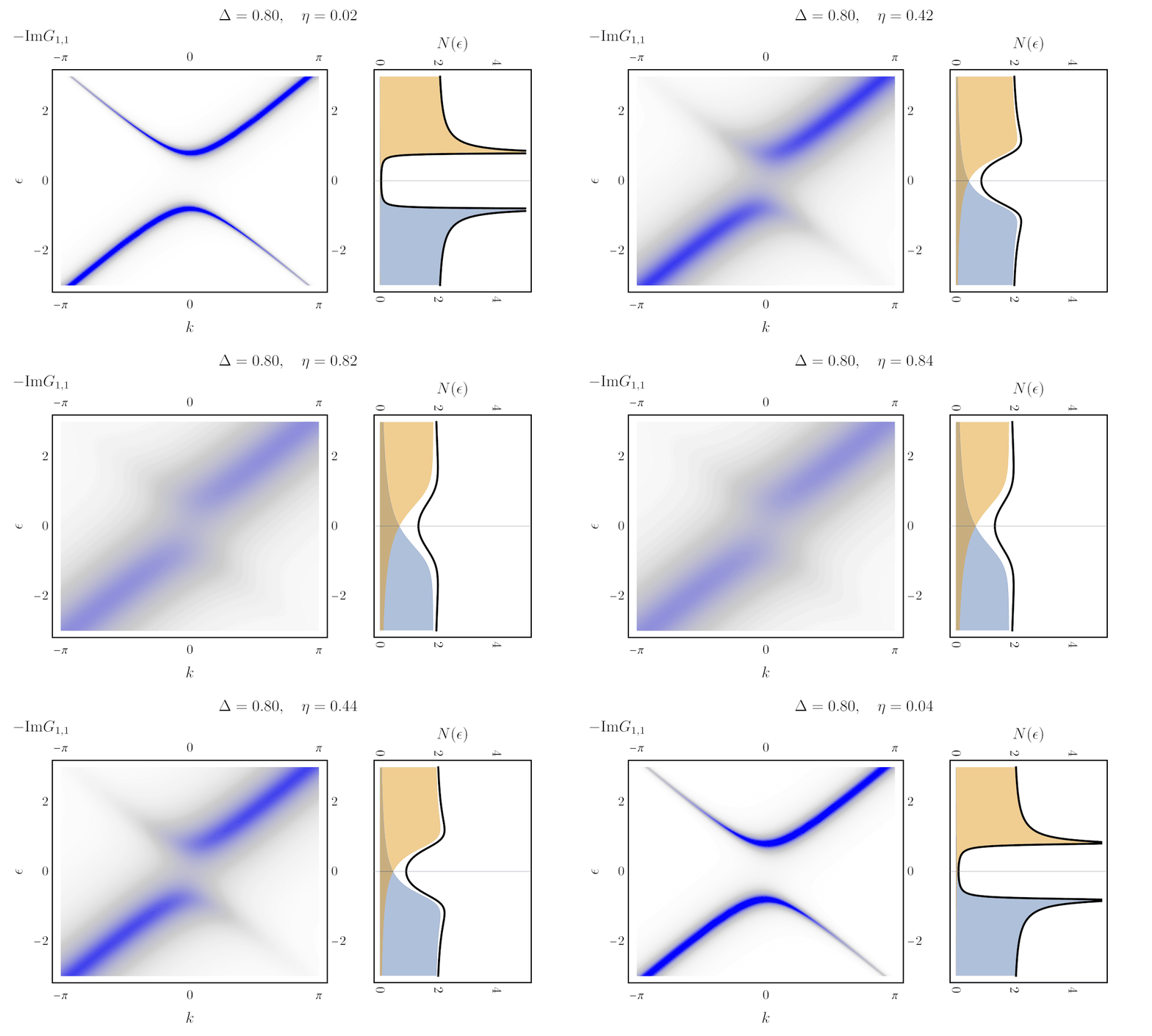
The total single-particle density of states (DOS), $D(\omega )$, which you know from your introductory condensed matter course, is simply the spectral function summed over all momenta:

To build a strong intuition for this relationship, let's explore it in the context of a simple tight-binding model. The following video explains how the spectral representation for a single non-interacting orbital (a delta function) broadens and combines with others to form the continuous density of states of a solid.

The video brilliantly illustrates how the formal definition of the spectral function connects to the familiar concept of the DOS. For a real, interacting system, the delta functions in the spectral function are broadened into peaks of finite width. The inverse of this width is a measure of the excitation's lifetime—a concept we will explore in detail later.

Finally, let's confirm this connection and mention a crucial sum rule with the help of our primary text resource.

Conclusion

This lesson has laid a critical piece of theoretical groundwork. We have moved from the specific framework of RPA to the much more general and powerful formalism of Green's functions.

Key Takeaways:

• The Lehmann representation is an exact, non-perturbative expression for the single-particle Green's function.
• The poles of the Green's function reveal the exact energies of single-particle (quasiparticle) excitations in the interacting system.
• The spectral function, $A(k,\omega )=-\frac{1}{\pi }\text{Im}{G}^R(k,\omega )$, gives the probability density of finding an excitation with momentum $k$ and energy $\omega$.
• The total density of states is the sum of the k-resolved spectral function over all momenta: $D(\omega )={\sum }_{k}A(k,\omega )$.
• The spectral function is normalized, satisfying the sum rule $\int d\omega A(k,\omega )=1$.

The Lehmann representation connects the Green's function we can calculate to the excitation spectrum we want to know. However, it is not a computational tool itself. The rest of this module will be dedicated to developing methods—namely, diagrammatic perturbation theory—to approximate the Green's function for interacting systems.

Preview of the Next Lesson

We have just established that the spectral function $A(k,\omega )$ is, in essence, the energy- and momentum-resolved map of allowed electronic states in a solid. In the next lesson, we will make this connection explicit by showing how $A(k,\omega )$ is precisely the quantity measured in Angle-Resolved Photoemission Spectroscopy (ARPES) experiments. This will firmly establish the spectral function as the primary bridge between many-body theory and one of the most powerful experimental probes of electronic structure.