Measuring Distributed Training Performance

Introduction

Welcome to the first lesson of our module on performance profiling and optimization. In the previous lesson, we grappled with the physical realities of large-scale AI systems, focusing on the immense power and cooling challenges presented by high-density GPU clusters. We established that these systems are not just computationally powerful but also incredibly expensive and energy-intensive.

This brings us to a critical question: how efficiently are we actually using all that hardware? Answering this requires a robust set of metrics to quantify performance. This lesson is dedicated to the learning outcome: Define key performance metrics for distributed training, including throughput (e.g., TFLOPs/s), hardware utilization (MFU/HFU), and scaling efficiency.

Understanding these metrics is fundamental for an AI systems designer. They are the language we use to measure success, diagnose problems, and guide optimization efforts. Without them, performance tuning is merely guesswork. By the end of this lesson, you will be able to define and reason about the core indicators of distributed training performance.

1. Throughput: Quantifying Computational Work

The most basic measure of performance is how fast a system completes a task. In the context of deep learning, the "task" is a vast number of mathematical calculations. The fundamental unit of this work is the floating-point operation, or FLOP.

As you saw, the core of a neural network's computation is math. To measure performance, we need to be precise with our terminology. Let's refine these definitions.

Let's consolidate these key definitions:

• FLOP (FLoating-point OPeration): A single arithmetic operation (add, subtract, multiply, divide) on floating-point numbers.
• MAC (Multiply-Accumulate): A compound operation, $a\times b+c$, common in neural networks. For accounting purposes, 1 MAC is considered equivalent to 2 FLOPs. Modern hardware often executes a MAC in a single clock cycle.
• FLOPS (FLoating-point Operations Per Second): A rate measuring computational performance. You will often see this expressed as GFLOPS ($10^9$), TFLOPS ($10^{12}$), or PFLOPS ($10^{15}$). This is analogous to measuring a car's speed in miles per hour.
• FLOPs (plural of FLOP): Refers to the total number of operations required for a task (e.g., "Training this model requires $10^{22}$ FLOPs"). This is analogous to measuring distance in miles. The ambiguity between FLOPS (rate) and FLOPs (total) is common, so context is key.

Throughput in TFLOP/s

While you could measure performance in "iterations per second," this metric is not portable. An "iteration" for a small model is computationally much cheaper than for a large one. A more universal metric is throughput, measured in TFLOP/s (TeraFLOPs per second).

Throughput (TFLOP/s) = (Total FLOPs per iteration) / (Time per iteration in seconds) / $10^{12}$

This metric tells you the actual computational throughput your system achieved during a training step. A higher TFLOP/s value is always better. To calculate it, you need two things: the total FLOPs per iteration and the time it took.

How do we determine the total FLOPs?

1. Estimation using Rules of Thumb: For transformer models, there are widely used formulas. A common approximation for the training FLOPs (forward + backward pass) is:
   $\text{FLOPs}\approx 6\times N\times D$
   where $N$ is the number of non-embedding parameters and $D$ is the total number of tokens processed. The factor of 6 comes from the forward pass costing $2\times N\times D$ FLOPs (a MAC operation per parameter) and the backward pass costing roughly twice that, so $2\times (2\times N\times D)=4\times N\times D$. Totaling $2+4=6$. If activation checkpointing is used (which we will discuss later), it adds another forward pass, making the formula $8\times N\times D$.

2. Automated Profiling: Modern frameworks can automatically count the FLOPs. As mentioned in the ml-engineering document (LINK), PyTorch provides torch.utils.flop_counter which can trace the execution of your model and give you a precise FLOP count. This is the preferred method for accuracy.

2. Utilization: MFU and HFU

Achieving a certain throughput, say 150 TFLOP/s, is a concrete number. But is it good? To answer that, you must compare it to the hardware's maximum capability. This brings us to the concepts of Model FLOPs Utilization (MFU) and Hardware FLOPs Utilization (HFU).

These metrics measure what fraction of the GPU's theoretical peak performance you are actually achieving.

Let's break this down:

• Theoretical Peak FLOPS: This is the number from the GPU's datasheet. For example, an NVIDIA H100 GPU has a theoretical peak performance of 989 TFLOPS for BF16/FP16 operations (using its Tensor Cores). This is your $100\%$ target.

• Hardware FLOPs Utilization (HFU):
  $\text{HFU}=\frac{\text{Actual Achieved TFLOP/s}}{\text{Theoretical Peak TFLOP/s}}$
  HFU measures the utilization based on all floating-point operations the GPU actually executed. This includes "useful" work like the model's forward and backward pass, as well as "extra" work from techniques like activation checkpointing (which re-runs the forward pass to save memory).

• Model FLOPs Utilization (MFU):
  $\text{MFU}=\frac{\text{Model-related TFLOP/s}}{\text{Theoretical Peak TFLOP/s}}$
  MFU is a more abstract metric. It considers only the "useful" FLOPs required by the model's forward and backward pass, ignoring any implementation-specific overhead like activation checkpointing. It answers the question: "Of the machine's total power, what percentage was spent on the core modeling task?"

Therefore, when activation checkpointing is used, HFU will be higher than MFU because HFU accounts for the re-computation FLOPs while MFU does not.

What is a "Good" MFU?

Achieving 100% utilization is impossible in a real-world training job due to data loading, communication overhead, non-matrix operations, and other system-level factors. So what should you aim for?

As a rule of thumb from the Stanford lecture slides (LINK), for large-scale training:

• MFU > 30% is considered good.
• MFU > 50% is excellent.

These targets give you a crucial benchmark for your optimization efforts. If your MFU is 15%, you know there is significant room for improvement. If it's 55%, you may be approaching the practical limits of the hardware and software stack.

Let's see this applied in a real-world cost estimation.

This example powerfully illustrates how MFU connects theoretical compute, real-world performance, and ultimately, cost. A lower MFU means you are paying for hardware that is sitting idle a larger fraction of the time. Maximizing MFU is a primary goal in distributed training.

3. Scaling Efficiency: Performance with More GPUs

Throughput and utilization metrics are vital, but they don't tell the whole story in a distributed setting. The crucial question is: how does your performance change as you add more GPUs? This is measured by scaling efficiency.

There are two fundamental ways to analyze scaling, which are beautifully illustrated in the following image.

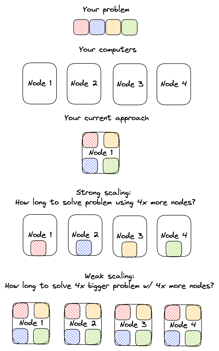
Let's define these in the context of distributed training:

• Strong Scaling: You have a fixed training task (e.g., train a 7B parameter model on 1 trillion tokens). You measure how the total training time decreases as you increase the number of GPUs from, say, 64 to 128 to 256.

  • Ideal Strong Scaling: Doubling the GPUs halves the training time.
  • Relevance: This is important when your goal is to reduce the time-to-solution for a fixed problem. It measures the system's ability to parallelize a constant amount of work.

• Weak Scaling: You fix the amount of work per GPU. For example, each GPU processes a local batch size of 8. As you increase the number of GPUs from 64 to 128, you also increase the global batch size from 512 to 1024. You then measure if the time per iteration remains constant.

  • Ideal Weak Scaling: Doubling the GPUs and doubling the workload keeps the time-per-iteration the same.
  • Relevance: This is important for measuring the system's ability to handle larger problems. It heavily stresses the communication network, as more GPUs need to synchronize more data.

In practice, scaling is never perfectly linear. Communication overhead (like the AllReduce operation for synchronizing gradients in data parallelism) and other synchronization bottlenecks mean that adding more GPUs yields diminishing returns. Scaling efficiency is the ratio of observed speedup to ideal linear speedup. An efficiency of 80% means you achieved 80% of the theoretical performance gain. As a systems designer, your goal is to choose parallelism strategies and network topologies that maximize this efficiency.

Conclusion

In this lesson, we have defined the essential vocabulary for measuring the performance of distributed AI training systems. You are now equipped to quantify performance and reason about efficiency at a professional level.

Key Takeaways:

• Throughput (TFLOP/s) is the most important measure of raw computational performance, normalizing for model size and hardware.
• MFU and HFU are critical utilization metrics that compare your actual throughput to the theoretical peak of your hardware. MFU, which measures "useful" model work, is the key metric to optimize, with >50% being an excellent target for large-scale jobs.
• Scaling Efficiency measures how effectively your system's performance increases as you add more GPUs. Understanding the difference between strong scaling (fixed problem, more GPUs) and weak scaling (growing problem, more GPUs) is crucial for evaluating distributed system performance.

Preview of the Next Lesson:

Now that we know what to measure, our next step is to learn how to diagnose performance issues. In the next lesson, we will explore the tools and techniques for performance analysis, addressing the learning outcome: Explain how to use profiling tools to identify if a workload is compute-bound, memory-bound, or communication-bound. This will move us from measurement to the first step of active optimization.