Reconstructing the Longest Common Subsequence

In our previous lesson, we established the core dynamic programming recurrence for the Longest Common Subsequence (LCS) problem and implemented a solution to find its length. We saw how the dp[i][j] table stores the optimal solutions to subproblems, with the final answer residing in the bottom-right cell.

Today, we will build directly on that foundation. Our goal is to move beyond just the length and learn how to reconstruct the actual LCS string. The DP table we built is more than just a collection of numbers; it's a map containing all the information we need. By tracing our decisions backward through this map, we can uncover the sequence of characters that form the LCS.

The Logic of Reconstruction: Backtracking Through Decisions

Think of the process of filling the DP table as a series of forward decisions. At each cell dp[i][j], we made a choice:

• If text1[i-1] == text2[j-1], we knew this character was part of the LCS for the current prefixes, and we took the result from the diagonal subproblem (dp[i-1][j-1]).
• If the characters differed, we took the best result from the preceding subproblems (dp[i-1][j] or dp[i][j-1]).

To reconstruct the LCS, we simply reverse this process. We start at the end—the bottom-right cell dp[m][n]—and trace our path back to the origin at dp[0][0]. The path we take reveals the characters that constitute the LCS.

The logic is a form of backtracking:

1. Start at (i, j) = (m, n).
2. If text1[i-1] == text2[j-1], we've found a character of the LCS. We add this character to our result and move diagonally to (i-1, j-1).
3. If text1[i-1] != text2[j-1], no character is added. We must determine which subproblem gave us the optimal value for dp[i][j]. We compare dp[i-1][j] (from above) and dp[i][j-1] (from the left) and move toward the larger value.
4. Repeat until we reach the edge of the table (i=0 or j=0).

The following article provides a crisp, formal explanation of this backtracking logic and presents it as clear pseudocode.

Visualizing the Backtracking Path

To make this process more concrete, let's watch how it's done. The following video walks through an example DP table and traces the path from the bottom-right corner, building the LCS string step by step.

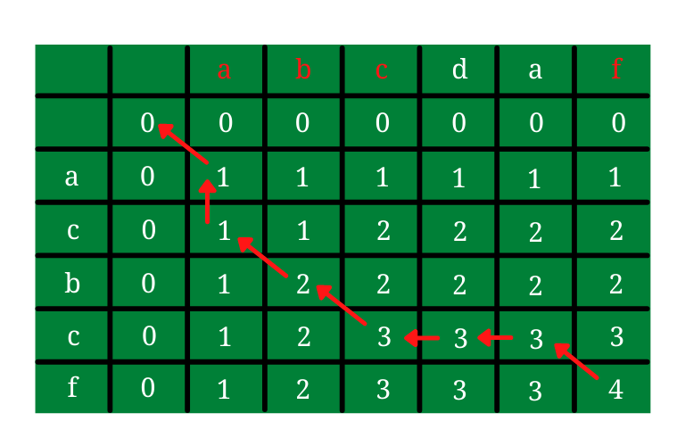
The path traced through the DP table might look something like this:

Implementation

Now, let's put it all together in code. The process involves two main parts:

1. Fill the (m+1) x (n+1) DP table exactly as we did in the previous lesson to find the length.
2. Implement a while loop that starts from (m, n) and backtracks to (0, 0), building the LCS string along the way.

The Programiz article below provides a clear and complete Python implementation that combines these two steps.

Here's a slightly modified version of that code for clarity, which uses a list to collect characters and then joins them, a common and readable pattern in Python.

def get_lcs_string(text1: str, text2: str) -> str:
    m = len(text1)
    n = len(text2)
    



    # 1. Fill the DP table (same as before)
    dp = [[0] * (n + 1) for _ in range(m + 1)]
    for i in range(1, m + 1):
        for j in range(1, n + 1):
            if text1[i-1] == text2[j-1]:
                dp[i][j] = 1 + dp[i-1][j-1]
            else:
                dp[i][j] = max(dp[i-1][j], dp[i][j-1])
    



    # 2. Reconstruct the LCS string by backtracking
    lcs_chars = []
    i, j = m, n
    
    while i > 0 and j > 0:



        # If characters match, this char is in the LCS
        if text1[i-1] == text2[j-1]:
            lcs_chars.append(text1[i-1])
            i -= 1  # Move diagonally up-left
            j -= 1



        # If not, move in the direction of the larger subproblem
        elif dp[i-1][j] > dp[i][j-1]:
            i -= 1  # Move up
        else:
            j -= 1  # Move left (or up if they are equal)
            



    # The characters were added in reverse order, so we reverse the list
    return "".join(reversed(lcs_chars))




# Example from the image
s1 = "abcdacf"
s2 = "acbcf"
print(f"The LCS of '{s1}' and '{s2}' is: '{get_lcs_string(s1, s2)}'") # Output: 'accf'

A quick note on complexity: filling the table takes $O(m\times n)$ time. The backtracking process, however, is much faster. In each step, we decrement either i, j, or both. This means the path from (m, n) to the edge of the table can be at most m + n steps long. Therefore, the reconstruction phase has a time complexity of $O(m+n)$.

What if Multiple LCS Strings Exist?

Consider the case where characters don't match, and dp[i-1][j] is equal to dp[i][j-1]. This indicates that there are at least two different paths that lead to the same optimal length. This means multiple, distinct LCS strings of the same maximum length can exist. Our algorithm, by convention (else: j -= 1), will always prefer one direction (e.g., moving left). This is perfectly acceptable; in an interview setting, you are typically only required to return one valid LCS.

Conclusion

In this lesson, we unlocked the full potential of the DP table we constructed for the LCS problem. We learned that by reverse-engineering the decisions made to fill the table, we can efficiently reconstruct the actual longest common subsequence.

Key Takeaways:

• Reconstruction via Backtracking: The core technique is to trace a path backward from dp[m][n] to dp[0][0].
• Path Decisions: The direction of movement at each step (i, j) is determined by comparing text1[i-1] and text2[j-1] and the values in the dp[i-1][j] and dp[i][j-1] cells.
• Diagonal Moves Yield Characters: A character is added to the LCS only when you make a diagonal move, which corresponds to a character match.
• Linear Time Reconstruction: The backtracking process is efficient, running in $O(m+n)$ time, which is subordinate to the $O(m\times n)$ time required to build the table.

The LCS pattern is highly versatile. In our next lesson, we will see how it can be cleverly adapted to solve a seemingly different problem: finding the Longest Palindromic Subsequence.