Recommended resources
The freely available resources this lesson will direct you to.
Welcome back. In our previous lesson, we examined the key components on a GPU specification sheet—Tensor cores, CUDA cores, and High Bandwidth Memory (HBM)—to understand a GPU's raw potential for LLM inference. We established that Tensor cores provide the computational horsepower, while HBM provides the memory capacity and bandwidth.
This lesson delves deeper into the memory aspect. The 80 GB of HBM on an H100 isn't a single, flat memory space. It's the largest and slowest tier in a complex GPU memory hierarchy. Your goal in this lesson is to understand this hierarchy and explain how the movement of data between its layers creates significant bandwidth bottlenecks, which are often the true performance limiters in LLM workloads. This is a core concept in LLM systems performance engineering.
1. The GPU Memory Hierarchy
In system architecture, a fundamental principle is the trade-off between memory speed, size, and cost. Memory that is extremely fast is also expensive and physically large, so you can only have a little of it. Memory that is large is cheaper but slower. GPUs, like CPUs, manage this trade-off using a memory hierarchy.
The closer memory is to the processing units (the SMs), the faster the access, but the smaller its capacity.
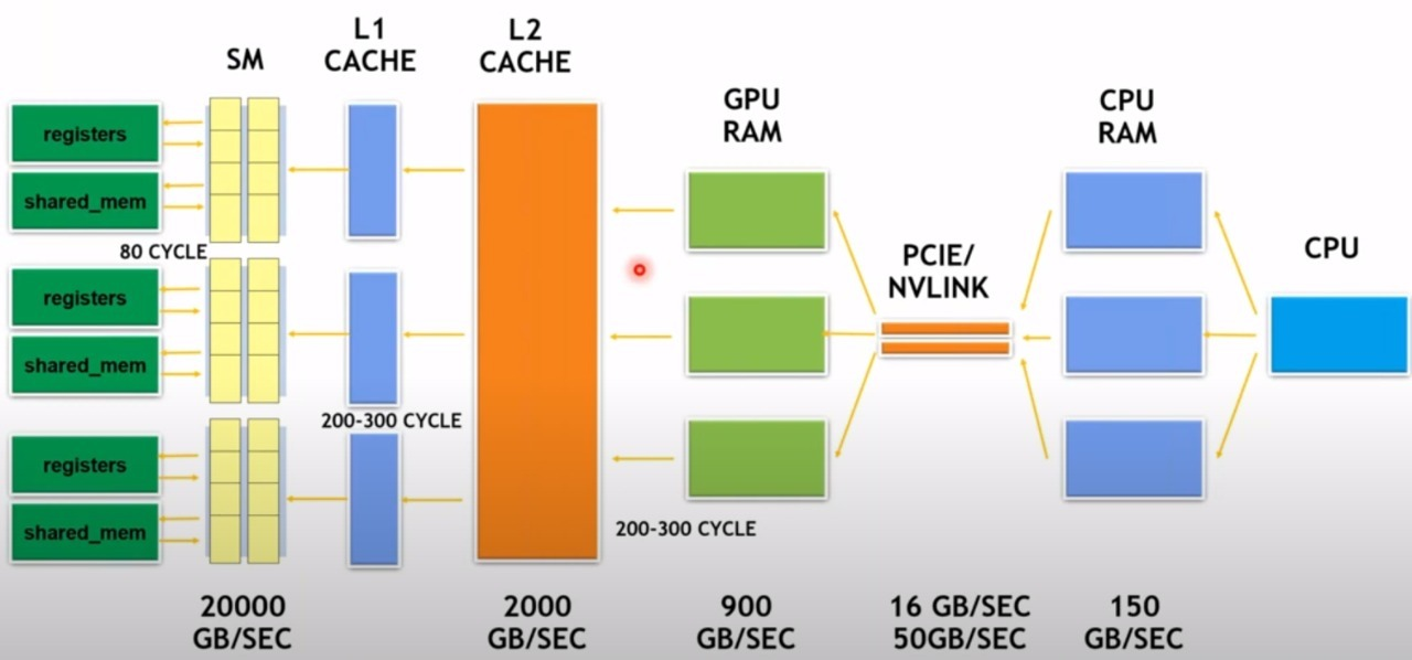
Let's walk through these layers, from fastest and smallest to slowest and largest. The following video provides an excellent programmer-centric overview of these memory types.
Memory Hierarchy | GPU Programming | Episode 6
This video from the "GPU Programming" series by Simon Oz explains the different types of memory available in CUDA, which directly map to the hardware's memory hierarchy.
Watch the following segments to understand each memory type's location and characteristics: On-chip vs. Off-chip: This establishes the fundamental physical separation that dictates memory speed. Registers: The fastest memory, located directly on the SM and private to each processing thread. Shared Memory: Fast, on-chip memory shared by threads within a block. This is often combined with the L1 cache. Global Memory: This is the main GPU memory (VRAM/HBM) we discussed previously. It's the largest but slowest, residing off-chip. Recap: A concise summary of all the memory types, their locations, and scopes.
To solidify this, the article below also provides a clear, hierarchical list.
Memory Bandwidth Engineering: The True Bottleneck in LLM GPU ...
This article from ObjectiveMind breaks down the key components of GPU architecture. We'll focus on its description of the memory hierarchy.
Read the subsection titled "Memory hierarchy significantly impacts overall performance" under the "Key components" heading. It provides a numbered list that neatly summarizes the hierarchy from registers to HBM.
Here is a summary of the GPU memory hierarchy, synthesized from these resources:
| Level | Location | Size | Speed / Latency | Role in LLM Inference |
|---|---|---|---|---|
| Registers | On-chip (SM) | Very Small (~256 KB/SM) | Fastest (~1 cycle latency) | Holds data for immediate computation by a single thread. |
| L1 Cache / Shared Memory | On-chip (SM) | Small (~128 KB/SM) | Very Fast (~30 cycles latency) | Caches frequently accessed data for threads in an SM. |
| L2 Cache | On-chip | Medium (~40-100 MB) | Fast (~200 cycles latency) | Shared cache across all SMs, reduces trips to HBM. |
| HBM (Global Memory) | Off-chip (Package) | Large (e.g., 80 GB) | Slowest (~800 cycles latency) | Stores model weights, optimizer states, and the KV cache. |
Your extensive background in infrastructure and SRE has likely involved diagnosing performance issues by analyzing I/O waits versus CPU utilization. The GPU memory hierarchy presents an analogous challenge: the phenomenal speed of the Tensor Cores is often gated by the time it takes to move data from the slow, off-chip HBM.
2. The Memory Wall: When Bandwidth is the Bottleneck
For decades, compute power has grown faster than memory bandwidth. This growing gap is known as the "memory wall." In the context of LLMs, which have model sizes in the tens or hundreds of gigabytes, this wall has become the primary performance bottleneck.
To understand why, let's watch a clip that explains how LLM inference constantly runs up against this wall.
How is hardware reshaping LLM design?
This video by Julia Turc, titled "How is hardware reshaping LLM design?", masterfully explains the memory bottleneck in LLM inference.
First, watch the introduction to the memory wall. It explains how model weights are stored in HBM and must be streamed to the on-chip processors (SRAM/SMs). Next, watch the crucial explanation of the bandwidth bottleneck. Pay close attention to the calculation performed. It demonstrates that even with the H100's impressive 3.35 TB/s of HBM bandwidth, the need to stream the entire model's parameters for every single generated token imposes a hard theoretical limit on token generation speed.
The key takeaway is that during autoregressive generation, the entire set of model weights must be read from HBM and streamed to the SMs to generate just one token. This process is repeated for every subsequent token.
This leads us to a critical distinction in systems performance: workloads can be either compute-bound or memory-bound.
- A compute-bound workload is limited by the processor's speed (FLOPS). The processor is running at 100% utilization while the memory system can keep up.
- A memory-bound workload is limited by the memory system's speed (bandwidth). The processor sits partially idle, waiting for data to arrive from memory.
As the video highlighted, LLM token generation is overwhelmingly memory-bound.
Arithmetic Intensity
To formalize this, we can use a metric called Arithmetic Intensity, defined as the ratio of floating-point operations (FLOPs) to the bytes of data moved from memory.
A high arithmetic intensity means you're doing a lot of computation for each byte you fetch, which is characteristic of a compute-bound task. A low arithmetic intensity means you're doing little computation for each byte, making you susceptible to memory bandwidth limits.
Memory Bandwidth Engineering: The True Bottleneck in LLM GPU ...
This article provides a great explanation of how to use arithmetic intensity to diagnose bottlenecks.
Read the entire section "Memory vs Compute: The Real Bottleneck?" This section defines arithmetic intensity and gives a clear rule of thumb for determining if a system is memory-bound or compute-bound by comparing the workload's intensity to the GPU's own hardware ratio. The example using Llama2-7B on an A10 GPU is a perfect illustration.
3. Prefill vs. Decode: Two Phases, Two Bottlenecks
The statement that LLM inference is memory-bound needs a crucial piece of nuance. As we briefly touched on in Module 1, inference happens in two distinct phases, and they have different performance characteristics.
- Prefill Phase: The input prompt is processed. All tokens in the prompt can be computed in parallel.
- Decode Phase: Output tokens are generated one by one, sequentially.

Because the prefill phase processes many tokens in parallel, it performs many computations for a single read of the model weights from HBM. This gives it a high arithmetic intensity, making it compute-bound. The GPU's Tensor Cores are typically fully utilized.
The decode phase, however, generates only one token at a time. For each token, it must read all the model weights and the growing KV cache from HBM. This results in a low arithmetic intensity, making the decode phase memory-bound.
The following resource explains this critical distinction with excellent clarity.
The Hidden Memory Architecture of LLMs
This article by Hazem Ali provides deep, systems-level insights into LLM memory behavior.
Read the section titled "LLM inference has two phases." It directly addresses why prefill is compute-heavy and decode is memory-hungry. The central idea is that decode performance is dominated by the time spent reading the KV cache from GPU memory, often leaving the compute units underutilized.
The phrase from the article, "When people ask why the GPU looks bored while tokens are slowly streaming, the answer is usually: Because decode is waiting on memory," is the single most important takeaway for understanding LLM inference performance. The bottleneck isn't the model's "thinking" time; it's the data transfer time dictated by the memory hierarchy.
Conclusion
In this lesson, we moved beyond a surface-level view of GPU memory and explored the hierarchy that governs its performance. You are now equipped to explain the primary bottleneck in most LLM serving scenarios.
Key takeaways from this lesson:
- GPUs have a memory hierarchy with different levels (Registers, L1/L2 Cache, HBM), each with a trade-off between speed and capacity.
- The relatively slow data transfer rate between the large off-chip HBM and the fast on-chip SMs creates a memory bandwidth bottleneck.
- LLM inference is a two-phase process: the prefill phase is typically compute-bound due to its high parallelism and arithmetic intensity.
- The token-by-token decode phase is severely memory-bound because it requires repeatedly streaming the model weights and KV cache from HBM to generate each new token, leading to low arithmetic intensity and underutilized compute cores.
In our next lesson, we will make these concepts tangible. You will learn to use the nvidia-smi command-line tool to monitor live GPU utilization, memory usage, and temperature, allowing you to observe the distinct resource signatures of the compute-bound prefill and memory-bound decode phases directly.