Decision Trees: Information Gain & Gini Impurity

Welcome to the first lesson in our module on advanced supervised learning methods. In the previous modules, we established a strong foundation in building and evaluating models like linear and logistic regression. These models operate by finding a single function—a line or a curve—that best fits the entire dataset. Now, we shift our focus to a fundamentally different and more intuitive class of models: decision trees.

Instead of a single global equation, a decision tree learns a hierarchical set of if/then rules, effectively partitioning the feature space into distinct regions. This approach is highly interpretable and mirrors human decision-making processes. Today, our objective is to understand the core algorithm that builds these trees. We will explore how a tree recursively selects the best features to split the data, using two key criteria: information gain (derived from entropy) and Gini impurity.

The Anatomy of a Decision Tree

At its heart, a decision tree is a flowchart-like structure. Given your background in computer science, you can think of it as a directed acyclic graph where nodes represent tests on features, edges represent the outcomes of these tests, and leaf nodes represent class labels. The process of using a tree for prediction is a simple traversal from the root to a leaf.

The video "Decision and Classification Trees, Clearly Explained!!!" provides an excellent overview of the structure of a tree and its basic terminology.

The fundamental challenge in building a decision tree is not the structure itself, but the algorithm for creating it. How do we decide which feature to use for the root node? And for each subsequent internal node, which split will be most effective? The answer lies in finding splits that progressively purify the data at each step.

The Recursive Algorithm for Building a Tree

The construction of a decision tree is an elegant application of a divide-and-conquer strategy, a concept you are undoubtedly familiar with from algorithm design. The general process is recursive:

1. Start with the entire dataset at the root node.
2. Select the best feature and split point to partition the data into two or more subsets. The "best" split is the one that results in the most "pure" child nodes.
3. For each child node, repeat the process with its subset of the data.
4. Stop splitting when a node is perfectly pure (contains samples from only one class) or when another stopping criterion is met (e.g., reaching a maximum depth or a minimum number of samples per node).

The core of this algorithm is step 2: how do we quantitatively define and measure the "purity" of a node to find the best split? This is where impurity metrics come into play. A perfect split would take a "mixed" or impure parent node and produce perfectly pure child nodes.

Measuring Impurity I: Entropy and Information Gain

One of the most important concepts for measuring impurity comes from information theory: Entropy. In this context, entropy is a measure of the uncertainty or disorder within a set of data points.

• A node with high entropy is very impure; it contains a mixed-up collection of different classes (e.g., 50% class A, 50% class B).
• A node with zero entropy is perfectly pure; it contains samples of only one class.

The video "Entropy (for data science) Clearly Explained!!!" provides a fantastic intuitive derivation of the entropy formula, starting from the idea of "surprise."

As the video explains, the Shannon Entropy for a node is calculated as the expected value of the surprise. For a set of classes $C$, where $p_i$ is the proportion of samples belonging to class $i$, the entropy $H$ is:

$$H(p)=-\sum _{i\in C}{p}_i{\log }_2(p_i)$$

When building a tree, our goal is not just to measure entropy, but to maximize the Information Gain from a split. Information Gain is simply the reduction in entropy achieved by partitioning the data on a particular feature.

For a dataset $D$ at a parent node, and a feature $A$ used for splitting, the information gain is:

$$\text{Gain}(D,A)=H(D_{\text{parent}})-\sum _{v\in \text{Values}(A)}\frac{|D_v|}{|D|}H(D_v)$$

Here, $D_v$ is the subset of data for which feature $A$ has value $v$. The second term is the weighted average entropy of the child nodes. The algorithm greedily chooses the feature split that yields the highest information gain.

Measuring Impurity II: Gini Impurity

While entropy is theoretically sound, its use of logarithms can be computationally intensive. An alternative and widely used metric is the Gini Impurity.

The Gini impurity of a node measures the probability of incorrectly classifying a randomly chosen sample from the node if it were randomly labeled according to the class distribution within that node. For a set of classes $C$, where $p_i$ is the proportion of samples of class $i$, the Gini impurity is:

$$\text{Gini}(p)=1-\sum _{i\in C}{p}_i^2$$

Like entropy, Gini impurity is 0 for a perfectly pure node and reaches its maximum for a 50/50 split in a two-class problem. The algorithm's goal when using this metric is to find the split that results in the lowest weighted average Gini impurity in the child nodes.

The following video provides a clear, step-by-step example of calculating Gini impurity to decide on the best split.

The process for a continuous feature, as shown in the video, involves sorting the feature's values and testing the midpoint between each adjacent pair as a potential split threshold. The threshold that yields the lowest impurity is chosen.

Gini vs. Entropy: A Comparison

You might wonder why there are two different metrics and which one to choose. In practice, they often produce very similar trees. The main difference is computational efficiency, with Gini being slightly faster as it avoids the log calculation.

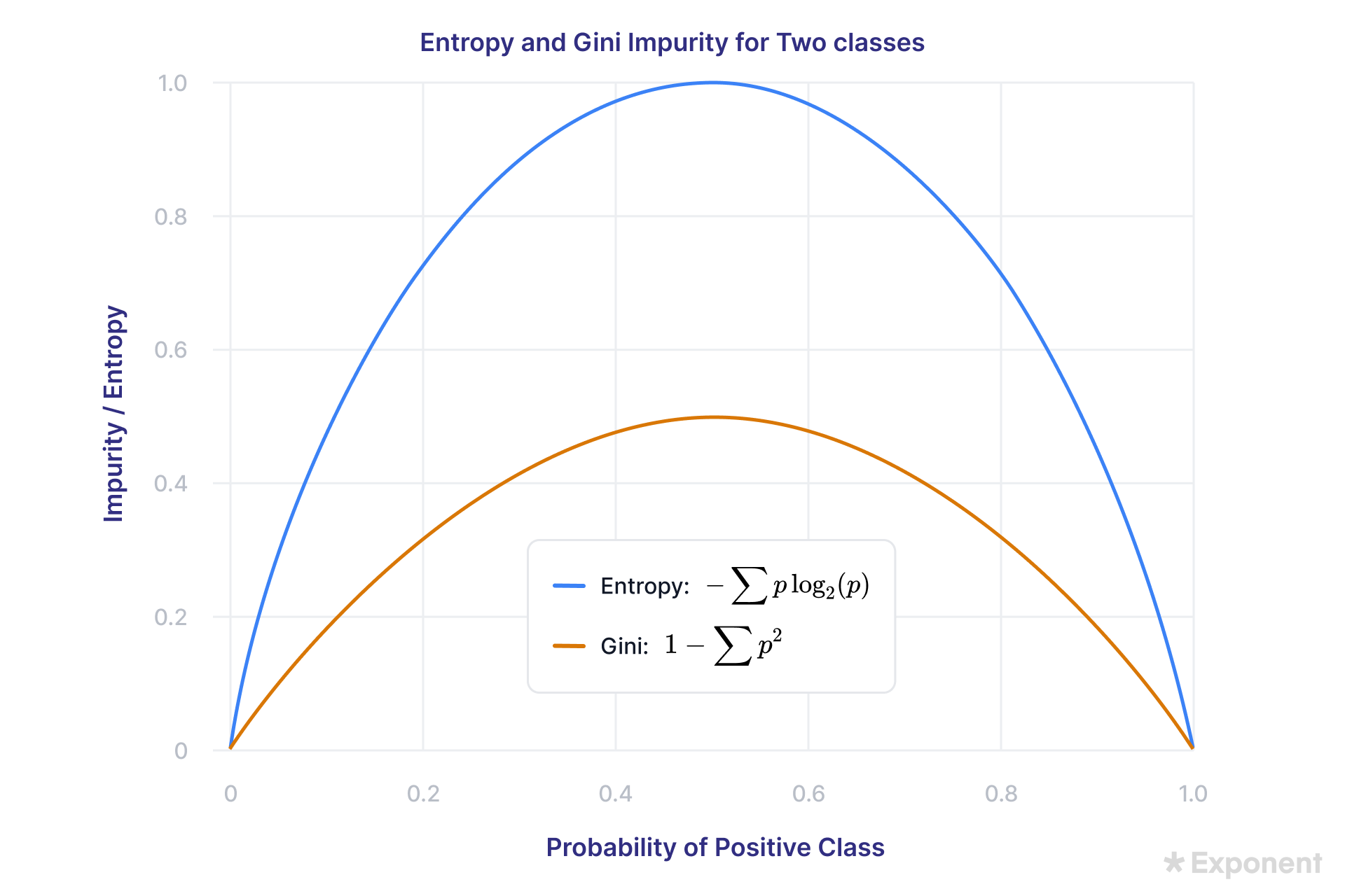
Let's consider a practical example.

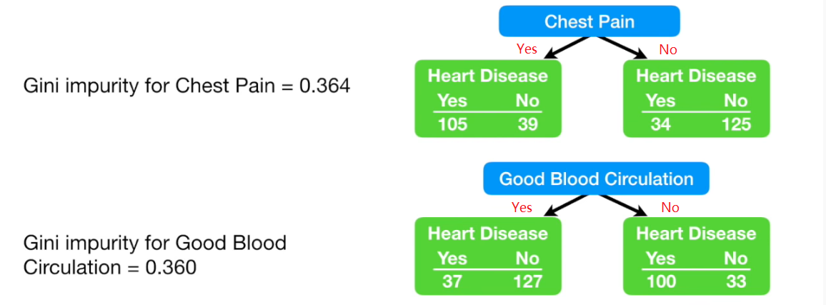
Based on the image above, the decision tree algorithm would choose the split on 'Good Blood Circulation' because its weighted Gini impurity (0.360) is lower than that of the split on 'Chest Pain' (0.364). This choice represents the most effective single step toward purifying the data.

A Deeper Theoretical Point: Why Not Misclassification Error?

A natural question arises: why use complex metrics like Entropy or Gini instead of the simple misclassification error?

$$\text{Error}(p)=1-\underset{i}{\max }(p_i)$$

The reason is that misclassification error is not sensitive enough to changes in the node's class probabilities. The following reading from Sebastian Raschka's lecture notes provides a compelling example where a split produces zero information gain when measured by misclassification error, but a positive gain when measured by entropy.

The concave nature of the entropy and Gini functions ensures that they favor splits that create purer nodes, even if those splits don't immediately change the majority class and thus don't reduce the immediate misclassification error. This property makes them better guides for the recursive partitioning algorithm.

Conclusion

In this lesson, we have dissected the fundamental algorithm behind decision trees. We've moved from a high-level, intuitive understanding of trees to the core mechanics of how they are constructed.

Here are the key theoretical takeaways:

• Decision trees are built using a recursive, divide-and-conquer algorithm that aims to create the purest possible leaf nodes.
• The "best" split at any node is determined by a splitting criterion that quantifies node impurity.
• Entropy measures the level of uncertainty or disorder in a node. The goal is to maximize Information Gain, which is the reduction in entropy after a split.
• Gini Impurity measures the probability of misclassifying a randomly selected element. The goal is to minimize the weighted Gini impurity of the child nodes.
• Both Entropy and Gini Impurity are preferred over simple misclassification error because their mathematical properties (specifically, their concavity) make them more sensitive to splits that improve node purity, guiding the tree towards a better overall structure.

While a single decision tree is powerful and highly interpretable, it has a significant drawback: it is highly prone to overfitting the training data. In our next lesson, we will explore Bagging and Random Forests, an ensemble technique that brilliantly combines many decision trees to create a far more robust and accurate model, directly addressing this weakness.