Interpreting Characteristic Curves: Exposure, Density, Contrast, and Dynamic Range

Hello. In the previous lesson, you followed an exposed silver-halide crystal through development, fixation, and washing. We now turn from the chemistry of an individual grain to the measured response of an entire processed emulsion. The characteristic curve tells us how much a negative darkens for a given exposure—and, just as importantly, where changes in exposure cease to produce useful differences in density.

This lesson focuses on black-and-white negative film. By the end, you should be able to read the curve’s axes and regions, extract a measure of contrast, and distinguish a film’s usable exposure range from the latitude available for a particular scene. Allow about 40 minutes, including the selected video and readings.

From a step exposure to a measured curve

Imagine exposing adjacent patches of one film strip to successively greater amounts of light, then processing the whole strip together. For constant image-plane illuminance $E$ and exposure time $t$, the exposure is

If $E$ is measured in lux, $H$ is in lux-seconds. The curve’s horizontal coordinate is usually the base-10 logarithm of exposure. More precisely, we can write $x={\log }_{10}(H/H_{\mathrm{ref}})$ for a chosen reference exposure; changing that reference merely shifts the horizontal labels. Doubling exposure moves a point by ${\log }_{10}2\approx 0.301$ horizontal units—the interval photographers call one stop.

After processing, a densitometer measures each patch’s transmission $T$, the fraction of incident measuring light that passes through it. Its optical density is

Thus $D=1$ transmits one tenth of the measuring light, while $D=2$ transmits one hundredth. Greater film exposure generally produces more developed image material, higher negative density, and lower transmission. This is the inversion to keep in mind: a bright part of the scene becomes a dark part of the negative.

Watch the selected portions of Basic Sensitometry, Part 1: The H&D Curve from The Naked Photographer for a concrete account of how the two plotted quantities are obtained. It is a demonstration of one film–developer combination, not a universal curve shape.

A characteristic curve is therefore not an intrinsic graph of silver halide alone. It describes a specified material under specified exposure, development, and density-measurement conditions. That qualification connects directly to the processing variables from the previous lesson.

Reading the toe, straight line, and shoulder

The Bureau of Standards paper Sensitometry of Photographic Emulsions gives a historical, quantitative account of density–exposure curves. Read its definition of density and its explanation of why a geometric series of exposures becomes convenient on a logarithmic axis. Some numerical labels in the scanned figures are difficult to read; the reasoning in the text is the useful part here.

The figure below is a schematic characteristic curve. Move from left to right as film exposure increases; move upward as the developed negative becomes denser.

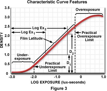
At very low exposures, the curve lies near its minimum density, $D_{\min }$. The film base is not perfectly transparent, and some density can arise without the intended image exposure—base plus fog, as the previous lesson’s chemistry would lead you to expect. The curve then bends upward through the toe. Here, a substantial change in exposure may yield only a small density difference. Scene shadows occupy this low-exposure part of a negative: a shadow can be recorded on the toe, but nearby dark tones become difficult to distinguish as the curve flattens toward $D_{\min }$.

Across the straight-line region, roughly equal changes in log exposure yield equal changes in density. This is the region of comparatively steady tonal separation, often associated with a scene’s midtones. “Straight” is an approximation over a finite interval, not a claim that the emulsion obeys one linear law at every exposure.

At sufficiently high exposure, some curves bend into a shoulder: density continues to increase, but by progressively less for each additional stop. These high-exposure parts of a negative correspond to scene highlights. A shoulder compresses highlight differences; it does not imply that every highlight entering it instantly loses all detail. Nor will every measured curve display a conspicuous shoulder within the exposures tested, as the video illustrates. $D_{\max }$ denotes the highest attainable density, but ordinary photographic measurements need not reach it.

Contrast is a slope, not a darkness

Suppose two patches receive exposures $H_1$ and $H_2$, both within the straight-line region. The region’s gradient, conventionally called gamma, is approximately

For example, if two patches one decade apart in exposure have densities 0.50 and 1.15, their straight-line gamma is $0.65$. A one-stop difference within that region then produces about $0.65\times 0.301\approx 0.20$ density units of separation. A steeper curve gives greater negative contrast: more density separation for the same scene exposure ratio. A dark negative is not necessarily a high-contrast negative; its overall density and its slope are different properties.

Away from the straight portion, the local gradient changes with position on the curve. Gamma alone cannot say how well two deep shadows separate on the toe or two bright highlights separate on the shoulder. It also cannot, by itself, describe the appearance of a finished print or scan, whose own tonal response matters.

Development changes the curve you measure. The same step exposures, developed for different times, can produce different densities and straight-line gradients. Read the original comparison in the Bureau of Standards paper; it gives experimental substance to the previous lesson’s statement that processing controls amplification rather than merely revealing a fixed final image.

Usable range depends on what you require from the image

To specify a usable exposure range, choose a lowest and highest exposure that still give adequate detail for the intended reproduction. Their separation on the horizontal axis is

The corresponding exposure ratio is $10^{\Delta x}$; in stops, the interval is $\Delta x/{\log }_{10}2$. For example, a usable width of $2.0$ log-exposure units represents a $100:1$ exposure ratio, or about $6.64$ stops.

The word usable carries a criterion. If you require nearly constant contrast, you might take only the straight-line interval. If reduced shadow or highlight separation is acceptable—and the print or scanner can recover it—you may include parts of the toe and shoulder. The full horizontal extent shown on a graph is therefore not automatically its usable dynamic range. Neither is the vertical difference $D_{\max }-D_{\min }$: that is a density interval, not an exposure ratio.

Kodak’s Basic Photographic Sensitometry Workbook is useful here for two practical distinctions: what sets the low-density baseline, and how a scene occupies only part of a film’s available exposure interval. Its conventions describe negative-film use, rather than imposing a single universal threshold for “usable.”

The older Bureau of Standards paper calls the range that can record a subject correctly the material’s scale, then reserves latitude for permissible variation in camera exposure for a particular subject. Its definition of “correctly” emphasizes placement on the straight-line region—a stricter criterion than merely obtaining a printable image.

Here is that interval argument in modern notation. Suppose your chosen usable film interval runs from $x=-2.0$ to $x=0.0$, while the darkest and brightest relevant scene areas span $1.5$ log units—a brightness ratio of about $32:1$, or five stops. If you place the scene’s shadows at $x=-1.8$, its highlights land at $x=-0.3$. The placement leaves $0.2$ log units before the shadow limit and $0.3$ before the highlight limit. You could reduce camera exposure by at most $0.2$ log units, or increase it by at most $0.3$, under those chosen usability limits. Those are approximately two-thirds of a stop of underexposure latitude and one stop of overexposure latitude.

Changing camera exposure shifts the whole scene interval horizontally; it does not shrink the scene’s brightness range. Consequently, latitude depends both on the film response and on the scene. A scene that nearly fills the usable interval leaves little room for error, even when the film itself has a substantial recording range.

Conclusion

A characteristic curve plots processed negative density against log exposure. Its toe records low exposures with diminishing shadow separation; its approximately straight region offers a fairly constant gradient; and a shoulder, when present, compresses high-exposure highlight differences. Gamma measures straight-line contrast, while the usable exposure range requires an explicit standard for adequate detail and reproduction. Latitude asks a different question: how far you can shift a particular scene’s exposures before some part falls outside that chosen range.

Next, we will examine why extending sensitivity or tonal performance is not free: grain size, resolving power, noise, and reciprocity behaviour all constrain how an emulsion can turn scarce photons into a useful record.