Finite-Size Scaling for Critical Exponent Ratios

Recommended resources

The freely available resources this lesson will direct you to.

[PDF] Monte Carlo tests of renormalization-group predictions for critical ...csml.northwestern.edu
[PDF] Resolving anomalies in the critical exponents of FePt using finite ...eprints.soton.ac.uk

Hello! Welcome to the final lesson of our module on computational methods for phase transitions.

In our previous lessons, we've built a complete workflow for analyzing a phase transition computationally. We've learned to run simulations with cluster algorithms, process the data with histogram reweighting, and, most recently, to pinpoint the critical temperature $T_{c}$ with high precision using the Binder cumulant method. With a reliable value for $T_{c}$ in hand, we are now ready for the final step: extracting the universal physics.

Today's learning outcome is to extract critical exponent ratios (e.g., $β / ν$ , $γ / ν$ ) by performing a data collapse using the finite-size scaling ansatz. This technique is not just a data analysis tool; it's a powerful, visual confirmation of the scaling hypothesis that lies at the heart of modern critical phenomena theory.

1. The Principle of Data Collapse

Let's recall the finite-size scaling (FSS) hypothesis for the magnetization $M$ and susceptibility $χ$ in a system of linear size $L$ . Near the critical point, they are expected to follow the forms:

M_{L} (t) = L^{- β / ν} \tilde{M} (t L^{1/ ν})

χ_{L} (t) = L^{γ / ν} \tilde{χ} (t L^{1/ ν})

where $t = (T - T_{c}) / T_{c}$ is the reduced temperature, and $\tilde{M}$ and $\tilde{χ}$ are universal scaling functions that are independent of the system's microscopic details.

The FSS ansatz makes a profound claim: although the raw data for $M_{L} (T)$ and $χ_{L} (T)$ look very different for different system sizes $L$ , there is a hidden unity. If we rescale the axes appropriately, all the data should fall onto a single, universal curve.

Specifically, if we plot the rescaled magnetization $M_{L} L^{β / ν}$ against the rescaled temperature $t L^{1/ ν}$ , the data from all system sizes should "collapse" onto the single master curve described by $\tilde{M} (x)$ . The same principle applies to the susceptibility.

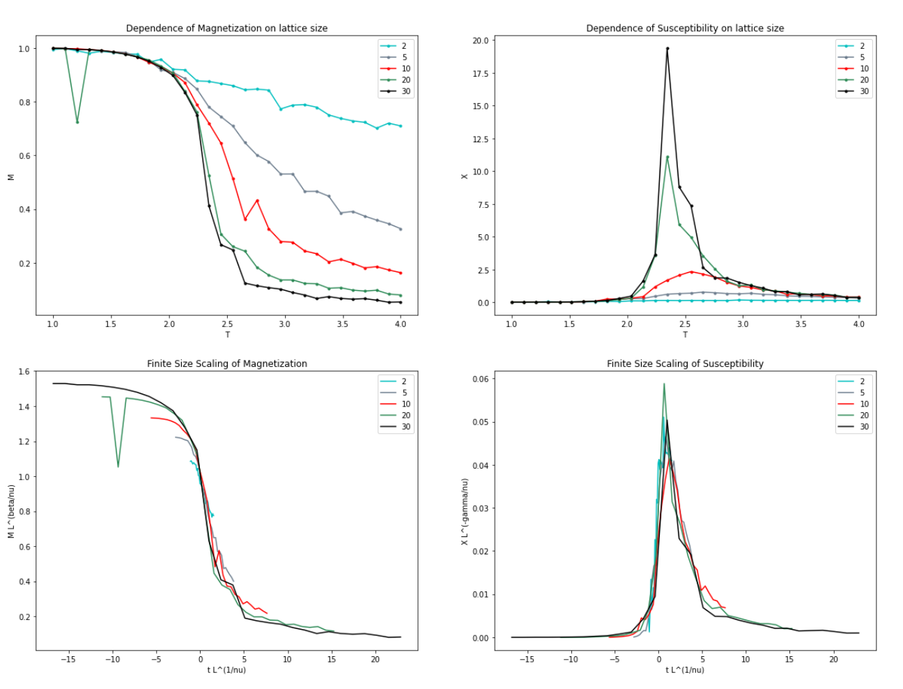
Finite-Size Scaling of Magnetization and Susceptibility — Top: Raw Monte Carlo data for magnetization (M) and susceptibility (X) vs. temperature (T) for various lattice sizes (L). Note how the transition sharpens as L increases. Bottom: The same data after rescaling the axes according to the FSS ansatz. The remarkable collapse of the data points onto single curves for both magnetization and susceptibility is a powerful confirmation of the scaling hypothesis. The exponents used for this collapse are the correct ones for the 2D Ising model ($\beta=1/8, \nu=1, \gamma=7/4$).

This procedure, known as data collapse, serves two purposes:

It is a stringent test of the scaling hypothesis.
It provides a method to determine the critical exponent ratios $β / ν$ , $γ / ν$ , and the exponent $1/ ν$ . The correct exponents are the ones that produce the best collapse.

2. Quantifying the Collapse: A Practical Method

"Best collapse" is a qualitative judgment. To implement this computationally, we need a quantitative measure of the quality of the collapse. The problem then becomes one of numerical optimization: finding the exponent values that minimize a "cost function" representing the scatter of the rescaled data.

A common method, adapted from a procedure developed by Bhattacharjee and Seno, is to calculate the average "distance" between the rescaled curves for all pairs of system sizes.

Resolving anomalies in the critical exponents of FePt using finite...

This paper by Waters et al. applies FSS to study the magnetism of FePt. While the physics is specific, the appendix provides an exceptionally clear and concise description of the data collapse algorithm we will use.

Please read Appendix A. Focus on understanding the definition of the minimization quantity P_b in Equation (7). Pay close attention to how it quantifies the difference between rescaled data curves from different system sizes, R_j and R_p. Also, note the extension to two variables in Equation (9), which generalizes the idea.

Let's break down the method described in the reading. For a set of magnetization curves $M_{j} (t)$ from systems of size $R_{j}$ , the cost function $P_{b}$ is essentially the mean-squared error between all pairs of rescaled curves:

P_{b} (β / ν, 1/ ν, T_{c}) = \frac{1}{N _{o l}} p \sum j \neq = p \sum i, o l \sum [R_{j}^{β / ν} M_{j} (t_{i}) - R_{p}^{β / ν} M_{p}^{*} (t_{i}^{*})]^{2}

Here:

The outer sums are over all pairs of system sizes $R_{j}$ and $R_{p}$ .
The term $R_{j}^{β / ν} M_{j} (t_{i})$ is a rescaled data point from the $j$ -th curve.
The term $R_{p}^{β / ν} M_{p}^{*} (t_{i}^{*})$ is a corresponding point from the $p$ -th curve. Since the rescaled temperature $t_{i}^{*} = (R_{j} / R_{p})^{1/ ν} t_{i}$ will not generally coincide with a simulation data point, an interpolated value $M_{p}^{*} (t_{i}^{*})$ from the $p$ -th dataset is used.
The inner sum is only over the range of temperatures where the rescaled curves overlap.
$N_{o l}$ is a normalization factor counting the total number of overlapping points.

Your task is to find the values of the exponents $β / ν$ and $1/ ν$ that minimize $P_{b}$ . Since you already have a high-precision estimate of $T_{c}$ from the Binder cumulant method, you can often hold it fixed during this minimization. This reduces the search space and makes the optimization more stable. This is a classic multi-dimensional minimization problem, solvable with standard numerical libraries (like scipy.optimize.minimize in Python). The exponent ratios that yield the minimum $P_{b}$ are your best estimates.

Test your understanding!

Suppose you are performing a data collapse for the magnetic susceptibility $χ$ . You write a script to minimize the corresponding cost function $P_{b}$ and find the best-fit values $γ / ν = 1.75$ and $1/ ν = 1.0$ . From this, what are your estimates for the individual exponents $γ$ and $ν$ ?

Show answer

From $1/ ν = 1.0$ , you can directly infer that $ν = 1.0$ .
Then, using $γ / ν = 1.75$ , you can find $γ$ by substituting your value for $ν$ :
$γ /1.0 = 1.75 ⟹ γ = 1.75$ .
These are the well-known exact values for the 2D Ising model.

3. Corrections to Scaling and Crossover Phenomena

In a real-world analysis, even with the correct exponents, the data collapse is rarely perfect. This is typically due to corrections to scaling. The FSS ansatz we've used represents only the leading-order asymptotic behavior for $L \to \infty$ . For finite $L$ , there are higher-order terms.

A more complete FSS expression, guided by renormalization group theory, looks like this for a generic quantity $A$ :

A_{L} (t) = L^{x_{A} / ν} [\tilde{A} (t L^{1/ ν}) + c_{1} L^{- ω} \tilde{A}_{1} (t L^{1/ ν}) + \dots]

Here, $ω > 0$ is a universal correction-to-scaling exponent, and the additional terms become less important as $L$ increases. These corrections cause the slight deviations from a perfect collapse that are often visible in practice, particularly when small system sizes are included in the analysis. For high-precision work, one might try to fit these correction terms as well, but this requires very high-quality data over a wide range of system sizes.

The idea of data collapse is even more powerful and can be generalized to describe crossover phenomena. Imagine a system where the nature of the interactions changes with a parameter, for instance, from short-range to long-range. The system might "cross over" from one universality class (e.g., Ising) to another (e.g., mean-field).

Monte Carlo tests of renormalization-group predictions for critical ...

The following is a highly detailed review article on Monte Carlo studies of critical phenomena. You are not expected to read it in its entirety. Instead, we will use it to look at examples of how the concept of data collapse is extended to more complex situations, which should be intellectually stimulating given your background.

Do not read this document. Just look at the figures I reference below. We will use them to see how data collapse works in more advanced scenarios.

Let's look at Figure 12 and Figure 15 in the document LINK.

Figure 12 shows a data collapse for a 2D Ising model where the interaction range $R$ is varied. The scaling variable is now $t R^{2}$ , which combines the temperature and the interaction range. The data for different $R$ values collapse onto a master curve that smoothly interpolates between the mean-field behavior (for large $t$ ) and the 2D Ising behavior (for small $t$ ).
Figure 15 shows a similar collapse for the 3D model. Here, the FSS variable is $χ L^{- γ / ν}$ vs. $L / R$ , showing a collapse that describes the crossover from a 3D bulk system to a zero-dimensional-like finite system.

These examples demonstrate the profound generality of scaling and data collapse. The scaling functions are not just abstract concepts; they are measurable master curves that govern the physics across different materials, system sizes, and even interaction types.

Conclusion

With this lesson, you have completed the computational toolkit for studying critical phenomena. You can now perform a full-cycle analysis: simulate a model, identify its critical point, and determine its universal critical exponents. This workflow is a cornerstone of modern research in statistical and condensed matter physics.

Key Takeaways:

Data collapse is the process of rescaling data for different system sizes so they fall onto a single, universal scaling function.
It serves as a direct, visual test of the finite-size scaling hypothesis.
The critical exponent ratios ( $β / ν$ , $γ / ν$ ) and the exponent $ν$ are the parameters that optimize the collapse.
This optimization can be automated by defining and minimizing a cost function that quantifies the "badness" of the collapse.
Deviations from a perfect collapse are often due to corrections to scaling, which are more prominent for smaller system sizes.
The principle of collapse can be generalized to describe more complex phenomena, like the crossover between different universality classes.

Preview of the Next Module:

Our journey through computational methods has provided concrete, numerical evidence for the abstract concepts of scaling and universality. We've seen data collapse. The natural question is: Why does this work? What is the deep physical principle that forces disparate systems to obey the same scaling laws near their critical points?

The next module, The Renormalization Group: Concepts and Real-Space Methods, will answer exactly that. We will delve into the revolutionary theoretical framework developed by Leo Kadanoff and Kenneth Wilson. You will see how the mathematical operation of data collapse is a direct reflection of the physical idea of "coarse-graining" and the flow towards a "fixed point" in the space of all possible Hamiltonians. This will provide the fundamental theoretical bedrock for everything we have observed in our simulations.