Excited-State Configuration Construction

Hello! Welcome back to our course on many-body quantum mechanics.

In our last lesson, we established that the Hartree-Fock (HF) mean-field theory, while a powerful starting point, is fundamentally limited because it describes a many-electron system with a single Slater determinant. This approximation neglects electron correlation, leading to significant errors in situations like bond dissociation and for the class of materials known as strongly correlated systems.

We concluded that to capture correlation, we must express the true wavefunction as a linear combination of multiple Slater determinants. Today, we'll address the essential next step: systematically generating these additional determinants. Our learning outcome is to construct excited-state configurations from a reference determinant for a many-electron system. This process is the bedrock of Configuration Interaction (CI) and other advanced post-Hartree-Fock methods.

1. The Starting Point: Occupied and Virtual Orbitals

Let's begin with the output of a standard Hartree-Fock calculation. For an $N$-electron system, we solve the HF equations using a basis set of $K$ spatial basis functions (e.g., atomic orbitals). This procedure yields a set of $K$ molecular spatial orbitals, and by including spin, we obtain a total of $2K$ spin-orbitals.

The Hartree-Fock ground state, which we call the reference determinant $|{\Phi }_0⟩$, is formed by filling the $N$ spin-orbitals with the lowest energies. These are the occupied orbitals. The remaining $2K-N$ higher-energy, unfilled spin-orbitals are called the virtual orbitals.

The core idea is that all other possible determinants can be generated by "promoting" or "exciting" electrons from the occupied orbitals into the virtual orbitals.

2. A Systematic Construction of Excited Determinants

Now that we have our two sets of orbitals—occupied and virtual—we can systematically construct all other possible $N$-electron Slater determinants. A standard and very useful notation is to use indices $a,b,c,\dots$ for occupied spin-orbitals and $r,s,t,\dots$ for virtual spin-orbitals.

Single, Double, and Higher Excitations

The different types of excited determinants are classified by the number of electrons that have been promoted from occupied to virtual orbitals.

Let's formalize this:

• Reference Determinant $|{\Phi }_0⟩$: The Hartree-Fock ground state.
• Singly Excited Determinants $|{\Phi }_a^r⟩$: Formed by replacing the occupied spin-orbital $a$ with the virtual spin-orbital $r$ in $|{\Phi }_0⟩$.
• Doubly Excited Determinants $|{\Phi }_{ab}^{rs}⟩$: Formed by replacing occupied spin-orbitals $a$ and $b$ with virtual spin-orbitals $r$ and $s$ in $|{\Phi }_0⟩$.
• Triply Excited Determinants $|{\Phi }_{abc}^{rst}⟩$: Formed by replacing $a,b,c$ with $r,s,t$.
• ...and so on, up to $N$-tuply excited determinants where all $N$ electrons are moved to virtual orbitals.

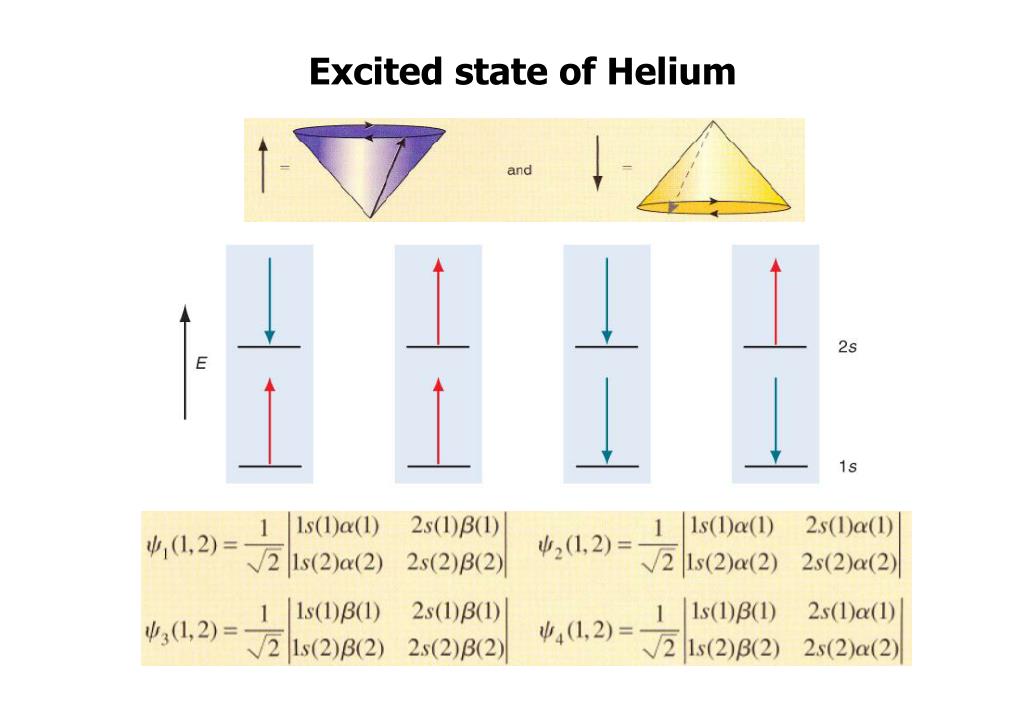
Let's visualize this with the Helium atom, which has $N=2$. The ground state is $1s^2$. An excitation promotes one electron from the $1s$ orbital to a higher-energy orbital, say the $2s$ orbital, resulting in a $1s^{1}2s^1$ configuration.

The Second Quantization Picture

Given your physics background, you'll appreciate that this process of creating excited determinants can be expressed very elegantly using the language of second quantization. The reference determinant $|{\Phi }_0⟩$ is our "vacuum" (in the sense that it contains no excitations). Excited determinants are created by applying creation (${\hat{a}}^{†}$) and annihilation ($\hat{a}$) operators to $|{\Phi }_0⟩$.

• $|{\Phi }_a^r⟩={\hat{a}}_r^{†}{\hat{a}}_a|{\Phi }_0⟩$ (annihilate an electron in state $a$, create one in state $r$)
• $|{\Phi }_{ab}^{rs}⟩={\hat{a}}_r^{†}{\hat{a}}_s^{†}{\hat{a}}_b{\hat{a}}_a|{\Phi }_0⟩$ (annihilate electrons in $a,b$, create them in $r,s$)

This formalism is not just a notational convenience; it is extremely powerful for deriving the matrix elements of the Hamiltonian between these determinants, which is a key step in actually solving the CI problem.

3. The Full Configuration Interaction (FCI) Expansion

The set of all possible determinants—the reference $|{\Phi }_0⟩$ plus all single, double, triple, ..., up to $N$-tuple excitations—forms a complete basis for the $N$-electron problem within the chosen one-particle basis set.

Therefore, we can write the exact many-body wavefunction, $|\Psi ⟩$, as a linear combination of all these determinants. This is known as the Full Configuration Interaction (FCI) expansion.

The FCI expansion is written as:

Here, the coefficients $c_a^r,c_{ab}^{rs},\dots$ are numbers that we need to determine. Finding these coefficients is the goal of a CI calculation. By using the variational principle to find the set of coefficients that minimizes the energy, we obtain the exact ground-state energy and wavefunction (within the limits of the one-particle basis set).

4. The Combinatorial Explosion and Practical Implications

At this point, it might seem like we've solved the many-body problem. We have a systematic way to construct a complete basis and a principle (the variational principle) to find the solution. However, there's a practical catch: the number of possible determinants grows astronomically with the size of the system.

As the video explains, the total number of determinants is $\left(\genfrac{}{}{0ex}{}{2K}{N}\right)$. This number grows factorially. For even a small molecule like water in a modest basis set, this number can be in the billions.

• Number of Singles $\sim O(N\cdot (2K-N))\sim O(K^2)$
• Number of Doubles $\sim O(N^2\cdot (2K-N{)}^2)\sim O(K^4)$
• Number of $m$-fold excitations $\sim O(K^{2m})$

This "combinatorial explosion" makes FCI computationally impossible for all but the smallest systems. This is the fundamental reason why a hierarchy of approximations exists. Most post-HF methods, like Configuration Interaction Singles and Doubles (CISD), involve truncating the FCI expansion at a certain excitation level (e.g., including only single and double excitations).

Conclusion

Today we've demystified the process of building the many-body wavefunction. By starting from the Hartree-Fock reference, we can systematically generate a complete basis of $N$-electron functions.

Key Takeaways:

• Solving the HF equations provides a set of occupied and virtual spin-orbitals.
• Excited determinants are constructed by promoting one or more electrons from occupied orbitals to virtual orbitals.
• These configurations are classified by their excitation level: Singles ($|{\Phi }_a^r⟩$), Doubles ($|{\Phi }_{ab}^{rs}⟩$), Triples, etc.
• The exact wavefunction (within a given basis) can be expressed as a linear combination of the HF reference and all possible excited determinants; this is the Full CI (FCI) expansion.
• The number of determinants grows combinatorially, making FCI computationally intractable for most systems and necessitating truncated CI methods.

Preview of the Next Lesson:

We now have the building blocks—the basis of Slater determinants. In the next lesson, we will put them to use. We will learn how to solve the Configuration Interaction (CI) problem for a minimal basis system. This will involve constructing the Hamiltonian matrix in our basis of determinants, $H_{IJ}=⟨{\Phi }_I|\hat{H}|{\Phi }_J⟩$, and diagonalizing it to find the correlated ground state energy and wavefunction. This will make the abstract concepts from the last two lessons concrete and calculable.