Recommended resources
The freely available resources this lesson will direct you to.
- Excel Cell Reference: Absolute, Relative or Mixed?www.youtube.com
- Switching between relative, absolute, and mixed references in Excel by Chris Menardwww.youtube.com
- Switch between relative, absolute, and mixed references | Microsoft Supportsupport.microsoft.com
- Absolute, Relative, and Mixed Cell References in Exceltrumpexcel.com
Hello! Last time, you imported a storefront CSV and confirmed that its four product-line records were in a structured Excel table. Now you’ll use those same numbers to make formulas that can be copied reliably.
In about 40 minutes, you’ll calculate line revenue, apply one shared commission rate, and build a grid of alternative rates. The central question is: when you copy a formula, which cell addresses should move, and which should stay put?
A reference describes what should move
Excel normally treats a cell reference as relative. If a formula in row 4 refers to B4, copying that formula one row down changes the reference to B5. That is useful when each product line needs its own calculation.
An absolute reference fixes both the column and row, as in $J$2. A mixed reference fixes just one: $D4 keeps column D fixed but allows the row to change; E$2 keeps row 2 fixed but allows the column to change. The dollar signs control copying behavior—they do not turn a value into currency or prevent someone from editing the referenced cell.
Watch Leila Gharani’s Excel Cell Reference: Absolute, Relative or Mixed? for the three situations in action.
Excel Cell Reference: Absolute, Relative or Mixed?
In “Excel Cell Reference: Absolute, Relative or Mixed?”, Leila Gharani demonstrates what happens when a working formula is filled into other cells—and how an initially plausible result can conceal a wrong reference.
Watch relative references as annual-total formulas move down rows. In absolute references, focus on why the denominator must remain at one cell and on the F4 shortcut. Finish with mixed references: notice why fixing both parts of a reference fails when the formula is copied down as well as across.
A useful way to predict any copied formula is to consider horizontal and vertical movement separately. Copying one cell right and one cell down would change these references as follows:
| Original reference | Copied reference | What stayed fixed? |
|---|---|---|
D4 |
E5 |
Nothing |
$D$4 |
$D$4 |
Column and row |
$D4 |
$D5 |
Column only |
D$4 |
E$4 |
Row only |
Build a small calculation sheet
Keep your StorefrontLines table from the previous lesson intact. Add a new, ordinary worksheet named ReferenceLab in the same workbook. We’re using ordinary cells here so you can see A1-style references clearly; formulas entered inside an Excel table may instead display structured references using column names.
Set up these cells on ReferenceLab:
- In
A3:H3, enter:LineID,Units,UnitPrice,LineRevenue,10%,15%,20%,StandardCommission. - In
A4:C7, enter the four lines below. Leave columns D through H empty for formulas.
| Row | A: LineID | B: Units | C: UnitPrice |
|---|---|---|---|
| 4 | L1 | 2 | 20 |
| 5 | L2 | 1 | 10 |
| 6 | L3 | 1 | 20 |
| 7 | L4 | 3 | 10 |
Put 10%, 15%, and 20% in E2, F2, and G2 respectively. Put Standard rate in J1 and 8% in J2. Enter rates with the % sign: typing 10 instead of 10% would make the calculation one hundred times too large.
Start with a relative formula. In D4, enter:
=B4*C4
Drag the fill handle—the small square at the selected cell’s bottom-right corner—down through D7. Inspect D5 in the formula bar: it should read =B5*C5. The results in D4:D7 should be 40, 10, 20, 30, matching the line revenues in your imported data. Both inputs needed to move to the next product line, so neither reference needed a dollar sign.
Keep one shared rate in place
Suppose the standard commission is 8% for every line. The revenue reference should change as you fill down, but the rate must always come from J2.
In H4, enter:
=D4*$J$2
Fill down through H7. You should get 3.2, 0.8, 1.6, 2.4. Inspect H7: its formula should be =D7*$J$2.
Why not use =D4*J2? When copied to H5, its rate reference would become J3, which is blank in this sheet. Excel might display a convincing-looking zero rather than the commission you intended. Locking both parts of $J$2 keeps every line tied to the same editable rate. On Windows, while editing a formula with the cursor on a reference, F4 cycles through the reference types; on some keyboards you may need Fn+F4. Typing the dollar signs yourself is equally valid.
Copy one formula across and down
Now the rate varies by column, while the product line varies by row. Read the “What are Mixed Cell References in Excel?” section of Absolute, Relative, and Mixed Cell References in Excel before building the grid.
Absolute, Relative, and Mixed Cell References in Excel
This TrumpExcel section uses a commission grid to explain why fixing only a column or only a row can be more useful than fixing an entire cell.
Find the heading “What are Mixed Cell References in Excel?”, after “When to Use Absolute Cell References in Excel?”. Begin at “Mixed cell references are a bit more tricky” and read the commission example through the explanation of E$2. Stop before “How to Change the Reference from Relative to Absolute (or Mixed)?”. Focus on what must change when copying right versus when copying down.
The resource’s example multiplies price and quantity within each grid formula. You have already calculated their product in column D, so your equivalent formula can be shorter. Enter this in E4:
=$D4*E$2
The two mixed references solve different problems. $D4 always takes revenue from column D, even when the formula moves right, but follows the current product-line row when it moves down. E$2 always takes a rate from row 2, even when the formula moves down, but follows the rate column when it moves right.
The image shows the longer version of this arrangement. Its formula fixes the price and quantity columns while allowing their row numbers to change; it fixes the rate row while allowing the rate column to change.
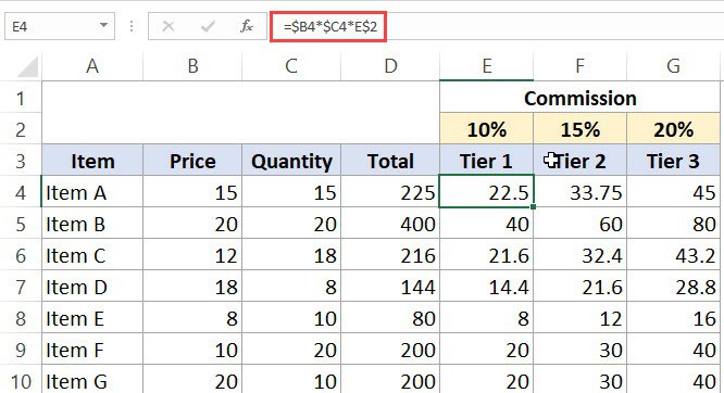
To fill your grid, drag E4 right through G4. Then select E4:G4 and drag the selection’s fill handle down through row 7. Check a few destinations rather than trusting the displayed values alone:
F4should be=$D4*F$2, giving 6.E5should be=$D5*E$2, giving 1.G7should be=$D7*G$2, giving 6.
If you had used D4 without locking its column, copying right would make it E4: the next commission would be calculated from the previous commission, not from line revenue. If you had used $D$4, every row would use L1’s revenue. Mixed references express the intended rule more precisely than either alternative.
Audit the behavior, not just the first answer
Before saving, inspect the formulas in both an adjacent column and a lower row. A formula can work in E4 yet fail elsewhere because its first position does not test copying. Confirm that D4:D7 holds 40, 10, 20, 30, H4:H7 holds 3.2, 0.8, 1.6, 2.4, and the far corner G7 refers to D7 and G2.
For one final check, temporarily change F2 from 15% to 16%. Values in column F should update—for example, F4 becomes 6.4—while columns E and G and the standard commission in H remain unchanged. Restore F2 to 15% afterward. This tests the business rule, not merely the appearance of the formula.
Key takeaways
Use a relative reference when an input should follow the formula’s new position, an absolute reference when every copy must use one cell, and a mixed reference when only the row or column should remain fixed. Predict copied formulas in both directions, then inspect a distant cell to verify your prediction.
Next, you’ll summarize business data with Excel aggregation functions. The reference choices you practiced here will also help you keep criteria and inputs pointed at the right cells when those summaries are copied.