Confusion Matrix and Performance Metrics

Hello! Let's embark on the next stage of our exploration into model evaluation.

In our previous lesson, we established a robust methodology—k-fold cross-validation—for obtaining a reliable estimate of a model's generalization performance. This solved the problem of how to measure performance without being misled by the randomness of a single data split. However, this process yields a "performance score," and we concluded by asking a critical question: what, precisely, should this score measure? For classification tasks, simply counting correct and incorrect predictions is often insufficient and can be dangerously misleading.

This lesson will address that question directly. We will deconstruct the performance of a classification model into its fundamental components using the confusion matrix. This simple yet powerful tool is the foundation for a nuanced understanding of a model's behavior. From this matrix, we will formally define and interpret the three most essential classification metrics: accuracy, precision, and recall. Understanding these metrics and their trade-offs is a pillar of applied machine learning, moving you from simply building models to rigorously evaluating and selecting them based on specific, real-world objectives.

Deconstructing a Classifier's Predictions

Before we can evaluate a classifier, we need a clear framework for categorizing its predictions. Many models, like the logistic regression we studied, don't output a class label directly. Instead, they produce a score or probability (e.g., the probability of belonging to the positive class). To turn this score into a concrete prediction (class 0 or 1), we must apply a threshold. For example, a common default is to classify an instance as positive if its probability is > 0.5, and negative otherwise.

Once this threshold is set, every prediction falls into one of four categories when compared against the true, ground-truth label. The following lecture from Stanford University provides an excellent introduction to this concept, showing how a score-based model becomes a classifier and how its predictions can be categorized.

As the lecture explained, the four outcomes are:

• True Positive (TP): The model correctly predicts the positive class. (e.g., correctly identifying a fraudulent transaction).
• True Negative (TN): The model correctly predicts the negative class. (e.g., correctly identifying a legitimate transaction).
• False Positive (FP): The model incorrectly predicts the positive class. This is also known as a Type I Error. (e.g., flagging a legitimate transaction as fraud).
• False Negative (FN): The model incorrectly predicts the negative class. This is also known as a Type II Error. (e.g., failing to detect a fraudulent transaction).

The distinction between False Positives and False Negatives is not merely academic; it is often the most critical aspect of evaluating a model. The "cost" of these two error types is rarely symmetrical in real-world applications. A blog post from Dataquest provides an excellent narrative to build intuition around this.

The Confusion Matrix: A Visual Summary

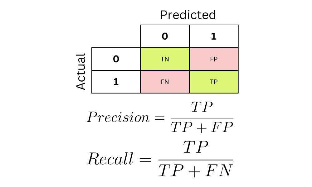
The confusion matrix is a table that organizes and summarizes the performance of a classification algorithm by tallying these four outcomes. It provides a holistic view of how the model's predictions align with the actual ground truth, showing exactly where the model is "confused."

The standard layout places the actual (true) classes along the rows and the predicted classes along the columns.

From this matrix, we can interpret performance in two ways:

1. Reading across the rows tells you what happened to each actual class. In the example above, for the "Actual Positive" row, we see that out of 40 sick people (30 TP + 10 FN), the model correctly identified 30 and missed 10.
2. Reading down the columns tells you about the reliability of the model's predictions. For the "Predicted Positive" column, we see that the model made 60 positive predictions (30 TP + 30 FP), of which only 30 were correct.

This two-way interpretation is what makes the confusion matrix an indispensable diagnostic tool.

Deriving Metrics from the Matrix

While the raw counts in the confusion matrix are informative, we need standardized, normalized metrics to compare different models or to evaluate performance against a business target. Accuracy, precision, and recall are the three most fundamental metrics derived directly from the TP, TN, FP, and FN counts.

The following academic paper provides concise, formal definitions for these metrics.

Let's dissect each metric in detail.

1. Accuracy

• Formula: $\text{Accuracy}=\frac{TP+TN}{TP+TN+FP+FN}$
• Question it answers: "Overall, what fraction of predictions did the model get right?"

Accuracy is the most intuitive metric. It simply measures the ratio of correct predictions to the total number of predictions. While simple, it can be a deeply flawed and misleading metric, especially when dealing with imbalanced datasets.

Consider a credit card fraud detection system where only 0.1% of transactions are fraudulent. A trivial model that predicts "not fraud" for every transaction would achieve 99.9% accuracy. While technically correct, this model is useless as it fails to identify any fraud at all. This "accuracy paradox" is why we need more nuanced metrics.

The Dataquest article provides a powerful illustration of this exact problem.

2. Precision

• Formula: $\text{Precision}=\frac{TP}{TP+FP}$
• Question it answers: "When the model predicts the positive class, how often is it correct?"

Precision measures the fidelity of positive predictions. It is the ratio of true positives to the total number of instances the model predicted as positive. A high precision score means that when the model flags an event, it is very likely to be a genuine event.

• When to prioritize Precision: When the cost of a False Positive is high.
  • Example: In email spam filtering, you want high precision for the "not spam" class. An FP here means a legitimate email is sent to the spam folder, which could be very costly (e.g., a missed job offer).
  • Example: In a recommendation system that suggests expensive products, a high-precision model ensures that the recommendations are highly relevant, avoiding user annoyance (a cost of FPs).

3. Recall (or Sensitivity)

• Formula: $\text{Recall}=\frac{TP}{TP+FN}$
• Question it answers: "Of all the actual positive instances, what fraction did the model successfully identify?"

Recall measures the model's ability to find all the relevant cases within a dataset. It is the ratio of true positives to the total number of actual positive instances. A high recall score means the model is effective at capturing the positive class and has a low number of false negatives. Recall is also widely known as Sensitivity or the True Positive Rate (TPR).

• When to prioritize Recall: When the cost of a False Negative is high.
  • Example: In medical screening for a serious disease, high recall is paramount. An FN means a sick patient is told they are healthy, with potentially fatal consequences. It is better to have some FPs (healthy patients who require further testing) than to miss a single case.
  • Example: In fraud detection, an FN means a fraudulent transaction is allowed to go through, resulting in a direct financial loss. Maximizing recall is crucial to minimize these losses.

This video from the codebasics channel provides a very clear, step-by-step visual explanation of how to calculate these metrics from a simple example.

The Inherent Trade-off

You may have noticed that precision and recall often pull in opposite directions. To increase recall, a model can be made more "liberal" by lowering its decision threshold. This will catch more true positives but will inevitably also generate more false positives, thus lowering precision. Conversely, to increase precision, the model can be made more "conservative" by raising its threshold. This ensures most positive predictions are correct but will cause it to miss more of the actual positive cases, lowering recall. This is known as the precision-recall trade-off, and it is a fundamental concept in classification.

Conclusion

In this lesson, we moved beyond a single, often misleading, performance number and developed a sophisticated framework for analyzing a classifier's behavior. The confusion matrix is not just a reporting tool; it is a diagnostic instrument that provides deep insight into a model's strengths and weaknesses.

Here are the essential takeaways:

• The confusion matrix categorizes all predictions into one of four outcomes: True Positives (TP), True Negatives (TN), False Positives (FP), and False Negatives (FN).
• Accuracy measures overall correctness but is a poor metric for imbalanced datasets due to the "accuracy paradox."
• Precision measures the reliability of positive predictions. It answers: "When my model says something is positive, how often is it right?" Prioritize it when False Positives are costly.
• Recall (Sensitivity) measures the completeness of positive detection. It answers: "Of all the true positive cases, how many did my model find?" Prioritize it when False Negatives are costly.
• The choice between prioritizing precision or recall is problem-dependent and should be driven by the real-world consequences of each type of error.

We are now equipped to have a much more meaningful discussion about model performance. However, we are left with a new challenge: how do we compare two models if one has higher precision and the other has higher recall? This leads directly to our next lesson, where we will explore the F1-score, a metric designed to summarize the precision-recall trade-off in a single number.