LLN and CLT: Cornerstones of Sampling

Recommended resources

The freely available resources this lesson will direct you to.

Introduction

In our previous lesson, we defined the theoretical properties of a probability distribution: its center of mass (expectation, $E [X]$ ) and its spread (variance, $V a r (X)$ ). These are abstract mathematical quantities. But in practice, whether in machine learning or computer graphics, we don't have access to the true, underlying distribution. Instead, we have data—a finite collection of samples.

A fundamental question arises: how does the sample average we compute from our data relate to the true, theoretical expectation? This lesson introduces two of the most profound and celebrated theorems in all of probability that answer this question: the Law of Large Numbers (LLN) and the Central Limit Theorem (CLT).

The LLN provides the foundational guarantee that as we collect more data, our sample average will indeed converge to the true expectation. This is the bedrock principle that makes sampling-based estimation possible. The CLT goes a step further, describing the shape and scale of the error in our estimate. It tells us that the distribution of the sample average itself follows a predictable and universal pattern. These theorems are not just theoretical curiosities; they are the justification for Monte Carlo methods, which are central to photorealistic rendering, and for the statistical inference that underpins nearly all of machine learning.

The Law of Large Numbers (LLN): Convergence to the Truth

The Law of Large Numbers formalizes the intuition that the average of a large number of independent and identically-distributed (i.i.d.) random trials should be close to the theoretical expected value.

Let's consider a sequence of i.i.d. random variables $X_{1}, X_{2}, \dots, X_{n}$ , all drawn from a distribution with mean $μ$ and variance $σ^{2}$ . The sample mean is defined as:

X ˉ_{n} = \frac{1}{n} i = 1 \sum n X_{i}

The LLN states that as $n$ gets very large, the sample mean $X ˉ_{n}$ converges to the true mean $μ$ . The following video from the Harvard Stat 110 course, taught by Prof. Joseph Blitzstein, provides a clear and intuitive explanation of this powerful concept.

Lecture 29: Law of Large Numbers and Central Limit Theorem | Statistics 110

This segment introduces the Law of Large Numbers, using the familiar example of coin flips to build intuition. It importantly contrasts the correct interpretation with the common misconception known as the "gambler's fallacy."

Please watch from the beginning of the LLN section. Focus on these key ideas: The Core Statement: The sample mean \bar{X}_n converges to the true mean \mu with probability 1 as n \to \infty. The "Swamping" Effect: Early-on random fluctuations (like a streak of heads) don't get "corrected" by an opposite streak. Instead, they are simply overwhelmed and rendered insignificant by the sheer volume of future trials. This is a crucial distinction. The Foundation of Science: The LLN is what makes empirical science possible. It guarantees that by collecting more data, we can get closer to the underlying truth of a phenomenon.

A First-Principles Proof of the LLN

To understand why the LLN holds, we can construct a proof for a slightly simpler version known as the Weak Law of Large Numbers. This version states that the probability of the sample mean being more than some small distance away from the true mean goes to zero as $n$ increases.

Before watching the proof, let's think. In the previous lesson, we saw that for i.i.d. variables, $V a r (X ˉ_{n}) = \frac{σ ^{2}}{n}$ . How might this fact—that the variance of the sample mean shrinks as $n$ grows—help us prove that $X ˉ_{n}$ gets closer to $μ$ ?

This shrinking variance is the key. The proof elegantly combines this property with Chebyshev's Inequality, which bounds the probability of a random variable being far from its mean, based on its variance.

Lecture 29: Law of Large Numbers and Central Limit Theorem | Statistics 110

This short segment provides a concise and powerful proof of the Weak Law of Large Numbers. It's a perfect example of how foundational concepts (variance, Chebyshev's inequality) combine to produce a profound result.

Watch the derivation from proving the weak law. Notice how the entire proof hinges on the fact that the variance of the sample mean has a 1/n term, which forces the probability bound to go to zero as n \to \infty.

The Central Limit Theorem (CLT): The Shape of Convergence

The LLN is powerful, but it only tells us that the sample mean converges to a single point. It doesn't tell us anything about the distribution of the sample mean for a finite $n$ . If we take $n = 100$ samples and compute the mean, and then repeat this experiment many times, how will our computed means be distributed? Will they be skewed? Uniformly scattered?

This is where the Central Limit Theorem comes in. It makes one of the most astonishing claims in all of science: regardless of the underlying distribution of the individual $X_{i}$ (as long as it has a finite variance), the distribution of the sample mean $X ˉ_{n}$ will be approximately a Normal (Gaussian) distribution for large $n$ .

This diagram illustrates the core idea of the CLT. The means of samples drawn from various distributions (bimodal, triangular, uniform, discrete, skewed) all result in a distribution that is approximately Normal (the bell curve).

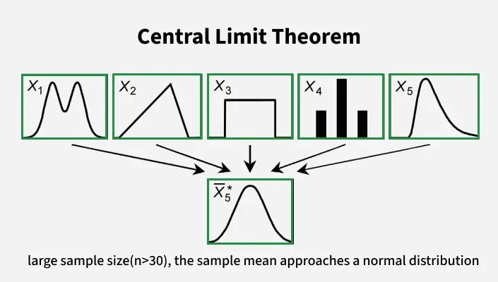
This explains why the Normal distribution appears so frequently in nature and statistics. Many observable quantities are the sum or average of numerous small, independent random effects, which is precisely the setup for the CLT.

The 3Blue1Brown video below provides a fantastic visual intuition for this process.

But what is the Central Limit Theorem?

This simulation-based explanation is ideal for building a strong mental model of the CLT. It shows how the process of summing random variables naturally gives rise to a bell curve.

Watch the segment from on dice roll simulations. Note how, even when starting with a highly asymmetric, weighted die, the distribution of the sum becomes more symmetric and bell-shaped as the number of dice in the sum increases.

Formal Statement of the CLT

The CLT is more precise than just saying the distribution looks "bell-shaped." It specifies the exact mean and variance of this resulting Normal distribution. Formally, for large $n$ , the sample mean $X ˉ_{n}$ is approximately Normal:

X ˉ_{n} \approx N (μ, \frac{σ ^{2}}{n})

To make this statement universal, we often look at the standardized sample mean. We subtract the mean and divide by the standard deviation to get a variable with a mean of 0 and a standard deviation of 1. The standardized sample mean is:

Z_{n} = \frac{X ˉ _{n} - μ}{σ / n}

The CLT states that as $n \to \infty$ , the distribution of $Z_{n}$ converges to the standard Normal distribution, $N (0, 1)$ .

The following segment from the Harvard lecture formally introduces the CLT, contrasting it with the LLN and highlighting the critical role of the $n$ scaling factor.

Lecture 29: Law of Large Numbers and Central Limit Theorem | Statistics 110

This video provides the precise mathematical statement of the CLT, distinguishing it carefully from the LLN.

Watch the segment from introducing the CLT. Focus on: The distinction: LLN is about the value \bar{X}_n converging to a constant \mu, while CLT is about the distribution of \bar{X}_n converging to a specific shape (Normal). The role of the \sqrt{n} scaling factor in stabilizing the variance so that the distribution converges to a non-degenerate form, rather than collapsing to a point (like in LLN) or blowing up.

The image below beautifully illustrates both theorems in action using a simulation of coin flips. As the number of flips n (the number in each subplot title) increases, the distribution becomes more tightly centered around the true mean of 0.5 (LLN) and its shape more closely resembles a perfect bell curve (CLT).

The distribution of the sample mean for an increasing number of fair coin flips, `n`. Each subplot shows a histogram of many computed sample means. As `n` increases, the distribution becomes more concentrated around 0.5 (LLN) and more bell-shaped (CLT).

A First-Principles Proof of the CLT

The proof of the CLT is more involved than that of the LLN, but it is a beautiful piece of mathematical reasoning. For a learner with your background, seeing it provides deep insight into why the Normal distribution is so special. The proof relies on showing that the Moment Generating Function (MGF) of the standardized sample mean converges to the MGF of a standard Normal distribution.

Lecture 29: Law of Large Numbers and Central Limit Theorem | Statistics 110

This segment walks through a full proof of the Central Limit Theorem using Moment Generating Functions (MGFs). This is a challenging but highly rewarding derivation that connects probability theory with calculus.

Watch the proof from Proving the CLT. Follow these key mathematical steps: The MGF of a sum of i.i.d. variables is the product of their individual MGFs. This leads to an MGF of the form [M(t/\sqrt{n})]^n, which results in the indeterminate form 1^\infty as n \to \infty. Taking the logarithm transforms the problem, allowing the use of L'Hopital's rule. Applying L'Hopital's rule twice, and using the properties of MGF derivatives at zero (M'(0) = \mu, M''(0) = E[X^2]), reveals that the log-MGF converges to t^2/2. This limit, e^{t^2/2}, is precisely the MGF of a standard Normal distribution, completing the proof.

Importance for Sampling and Computer Graphics

So, what is the practical importance of these theorems? They are the theoretical justification for almost all sampling-based estimation. This is especially relevant to your interest in computer graphics.

Techniques like Monte Carlo path tracing, used to render photorealistic images, work by estimating an integral—the rendering equation—which represents the total light arriving at a pixel. This integral is estimated by averaging the contributions of many random light paths traced through the scene.

The LLN guarantees that this process works. It ensures that as we trace more and more rays (n increases), our estimate of the pixel's color ( $X ˉ_{n}$ ) will converge to the true, correct color ( $μ$ ).
The CLT tells us the rate of convergence and the nature of the error (noise). The standard deviation of our estimate, often called the standard error, is $σ / n$ . This means the visual noise in a rendered image decreases in proportion to $1/ n$ .

This $1/ n$ relationship is a fundamental law in rendering. Based on this, what must you do to the number of samples (rays per pixel) to cut the amount of noise in half?

Answer

To halve the error (standard deviation), you must divide $\sigma/\sqrt{n}$ by 2. This is equivalent to putting a factor of 4 inside the square root: $\sigma/\sqrt{4n}$. Therefore, you must **quadruple** the number of samples. This is why rendering high-quality, noise-free images can be so computationally expensive.

The following text connects these ideas formally within the context of Monte Carlo estimation.

Mathematical Basics of Monte Carlo Rendering Algorithms

This document explicitly links the abstract theorems we've discussed to the concrete problem of Monte Carlo integration, which is the engine behind modern photorealistic rendering.

Please read Section 2.4, focusing on the subsections A Monte Carlo Estimator and Variance of the Estimator. Pay special attention to how: The problem of computing an integral is reframed as computing an expectation. The LLN justifies using the sample average (the "Monte Carlo estimator") to approximate this expectation. The CLT quantifies the error of this estimator, explicitly stating that the standard deviation varies as 1/\sqrt{N}. This is the mathematical origin of the noise reduction rule in rendering.

Conclusion

Today we explored two of the most critical theorems in probability theory, which bridge the gap between abstract distributions and practical data analysis.

Key Takeaways:

Law of Large Numbers (LLN): Guarantees that the sample average of i.i.d. variables converges to the true expected value as the sample size grows infinitely large. This is the foundation of estimation by sampling.
Central Limit Theorem (CLT): States that the distribution of the sample average (properly standardized) approaches a standard Normal distribution, regardless of the original distribution's shape. This is a statement about universality.
Importance for Sampling: The LLN validates sampling as a method for estimation. The CLT quantifies the error in that estimation, showing that the standard error decreases in proportion to $1/ n$ . This rule governs the trade-off between computational cost and accuracy in fields from machine learning to computer graphics.

Preview of the Next Lesson:

The LLN and CLT are cornerstones of the "frequentist" school of statistics, which focuses on the long-run behavior of sample averages. In our next lesson, we will pivot to a different, powerful paradigm for reasoning under uncertainty: Bayesian inference. We will introduce Bayes' Theorem and explore how it provides a formal framework for updating our beliefs about the world as we acquire new evidence. This shift in perspective is fundamental to many advanced topics in AI, including probabilistic models and generative AI.