Barometric Formula Derivation for Isothermal Atmospheres

Hello! Welcome back.

In our previous lesson, we established the principle of hydrostatic equilibrium, which describes the balance between gravity and the pressure gradient force. This led us to a fundamental differential equation describing the vertical structure of the atmosphere:

$\frac{dP}{P}=-\frac{g}{R_{\text{specific}}T}dz$

This equation tells us that the fractional change in pressure with height depends on temperature. To find the actual pressure profile, $P(z)$, we need to solve this equation.

Today's lesson directly follows from this point. We will tackle the learning outcome: to derive the barometric formula to show how atmospheric pressure decreases exponentially with altitude in an isothermal atmosphere. To do this, we will make a simplifying assumption about the atmosphere's temperature structure, solve the differential equation, and analyze the result.

This is a classic problem in atmospheric physics, and the resulting formula provides the first quantitative approximation of the atmosphere's pressure profile.

1. The Isothermal Atmosphere Assumption

To integrate the equation $\frac{dP}{P}=-\frac{g}{R_{\text{specific}}T}dz$, we need to know how temperature $T$ behaves as a function of altitude $z$. The simplest possible assumption is that the temperature is constant.

An isothermal atmosphere is a model atmosphere where the temperature does not change with altitude ($T(z)=\text{constant}$).

While we know from experience (e.g., climbing a mountain) that this is not strictly true for the real atmosphere, it serves as a powerful first approximation. By assuming $T$ is constant, along with our previous reasonable assumptions that $g$ and $R_{\text{specific}}$ are also constant, the term $\frac{g}{R_{\text{specific}}T}$ becomes a single constant value. This transforms our problem into a simple, first-order ordinary differential equation that you'll likely find familiar from your previous studies in mathematics.

2. Deriving the Barometric Formula

With the isothermal assumption in place, we can now integrate the hydrostatic equation to find $P(z)$. The following resource provides a clear, step-by-step derivation. While it starts from the initial force balance, which we covered last lesson, it's useful to see the full logical flow from forces to the final exponential formula.

Let's summarize the key mathematical steps of the integration you just reviewed:

1. Start with the differential form:
   $\frac{dP}{P}=-\frac{g}{R_{\text{specific}}T}dz$
   Here, we use $z$ for altitude, which is equivalent to $h$ in the reading.

2. Integrate both sides: We integrate from a reference level (altitude $z_0$, pressure $P_0$) to an arbitrary altitude $z$ where the pressure is $P(z)$. Since $g$, $R_{\text{specific}}$, and $T$ are assumed constant, the term on the right can be moved outside the integral.
   ${\int }_{P_0}^{P(z)}\frac{dP}{P}=-\frac{g}{R_{\text{specific}}T}{\int }_{z_0}^{z}dz$

3. Evaluate the integrals: The integral of $1/P$ is $\ln (P)$, and the integral of $dz$ is just $z$.
   $[\ln (P){]}_{P_0}^{P(z)}=-\frac{g}{R_{\text{specific}}T}[z{]}_{z_0}^z$
   $\ln (P(z))-\ln (P_0)=-\frac{g}{R_{\text{specific}}T}(z-z_0)$

4. Solve for $P(z)$: Using the logarithmic identity $\ln (a)-\ln (b)=\ln (a/b)$, we get:
   $\ln \left(\frac{P(z)}{P_0}\right)=-\frac{g}{R_{\text{specific}}T}(z-z_0)$
   Exponentiating both sides gives the Barometric Formula:
   $P(z)=P_0\exp \left[-\frac{g}{R_{\text{specific}}T}(z-z_0)\right]$

This equation shows that in an isothermal atmosphere, pressure decreases exponentially with height.

3. Scale Height

The barometric formula can be written in a more compact and intuitive form by introducing a new term called the scale height, usually denoted by $H$.

The scale height is defined as:
$H=\frac{R_{\text{specific}}T}{g}$
Notice that $H$ has units of length (e.g., meters or kilometers). Substituting this into the barometric formula gives:
$P(z)=P_0{e}^{-(z-z_0)/H}$

What does $H$ represent physically?
It is the characteristic vertical distance over which the atmospheric pressure decreases by a factor of $1/e$ (approximately 37%). If you move upward by one scale height, $z-z_0=H$, the pressure drops to $P_0/e$.

The following resource provides a concise derivation similar to the one above and introduces the scale height concept very clearly.

For a typical Earth surface temperature of $T\approx 290$ K, the scale height is about 8.8 km. This means that at an altitude of 8.8 km (roughly the height of Mount Everest), the atmospheric pressure is about $1/e$ times the pressure at sea level.

4. Visualizing the Result and Evaluating the Model

The exponential decay predicted by the barometric formula is a fundamental feature of our atmosphere. The graph below shows this relationship.

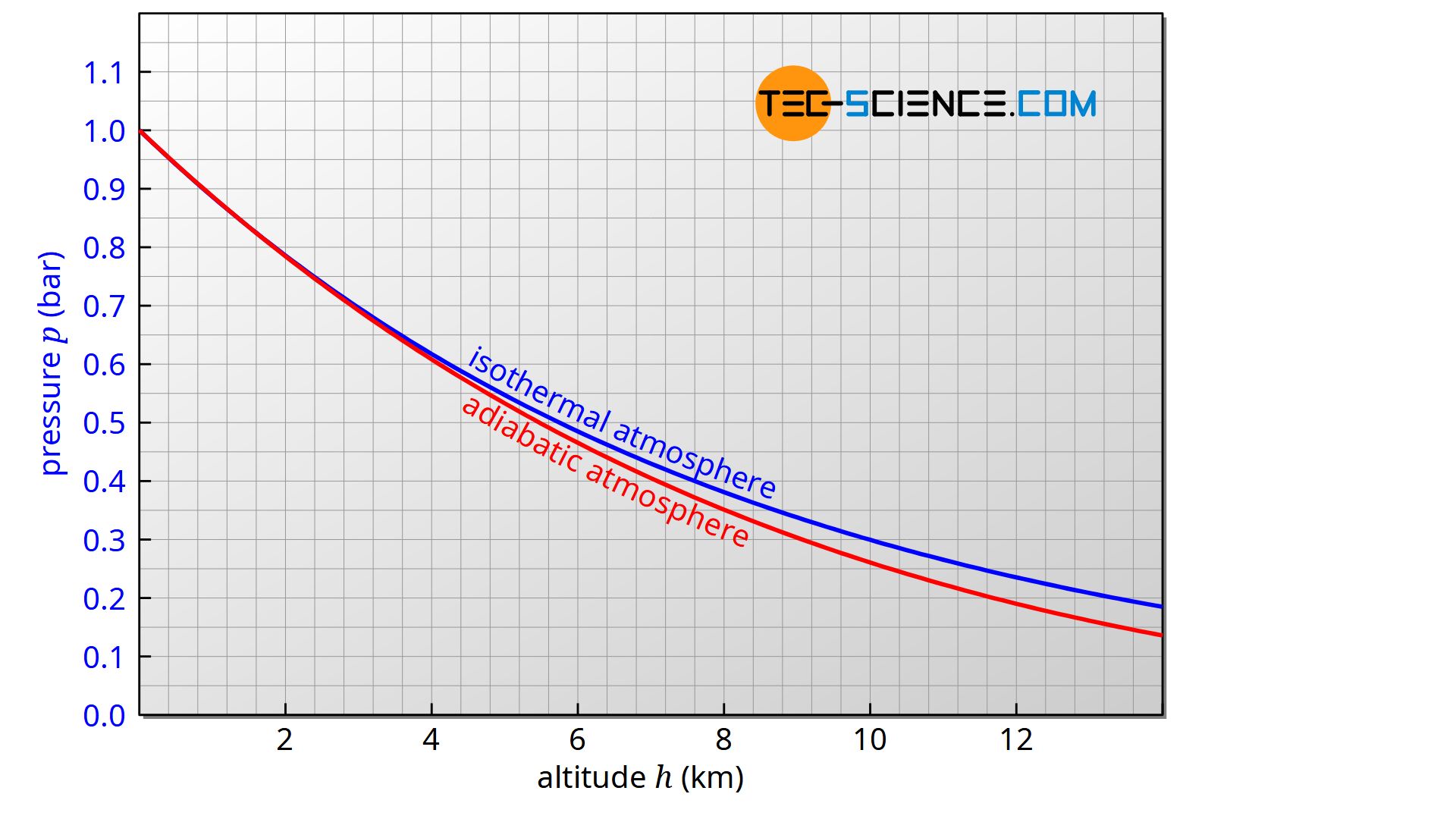
The blue curve is a plot of our result, $P(z)=P_0{e}^{-z/H}$. As you can see, the pressure drop is rapid at first and becomes more gradual at higher altitudes, which is characteristic of exponential decay.

However, our derivation rested on a major simplification: a constant temperature. How good is this assumption? For a model to be useful, we must understand its limitations.

As the reading explains, the isothermal assumption is a significant simplification. In the troposphere (the lowest ~10-15 km of the atmosphere), temperature actually decreases with height. This has a noticeable effect on the pressure profile, as shown by the difference between the blue (isothermal) and red (adiabatic) curves in the graph above. The pressure in a more realistic model of the troposphere drops faster with height than in the isothermal case.

Conclusion

In this lesson, we have built upon the concept of hydrostatic equilibrium to develop a quantitative model of the atmosphere's pressure structure.

Key Takeaways:

• By assuming a constant temperature (isothermal atmosphere), the hydrostatic balance equation can be solved.
• The solution is the barometric formula: $P(z)=P_0{e}^{-(z-z_0)/H}$, which shows that pressure decreases exponentially with altitude.
• The scale height, $H=R_{\text{specific}}T/g$, is the characteristic altitude increase over which pressure drops by a factor of $1/e$. For Earth, $H$ is approximately 8-9 km.
• The isothermal model provides a good first approximation but deviates from reality because the actual atmospheric temperature is not constant with height.

Preview of the Next Lesson:

We have now seen the consequences of assuming a constant temperature. The next logical step is to relax this assumption and build a more realistic model. In the next lesson, we will use the first law of thermodynamics in conjunction with the hydrostatic equation to derive the dry adiabatic lapse rate, which describes how the temperature of a rising parcel of dry air changes with altitude. This will explain the physics behind the red curve in the graph and give us a more accurate picture of the atmosphere's thermal structure.