Understanding Algorithmic Efficiency: Best, Worst, and Average Cases

Welcome back! In our last lesson, we developed a practical toolkit for determining the time complexity of iterative code. We learned to analyze loops and conditional statements, often implicitly focusing on the scenario that takes the longest to run.

Today, we will formalize and expand upon that idea. We'll explore how an algorithm's efficiency isn't a single, fixed value but can change dramatically based on the specific input it receives. To understand this, we will distinguish between best-case, worst-case, and average-case analysis. This will add a crucial layer of nuance to our ability to describe and compare algorithm performance.

Defining the Scenarios

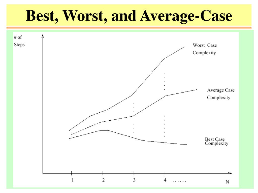
When we analyze an algorithm for a given input size, n, we are interested in three distinct performance scenarios.

• Best-Case Analysis: This measures the minimum number of operations an algorithm takes for any input of size n. It represents the "luckiest" possible input that allows the algorithm to finish in the shortest amount of time.
• Worst-Case Analysis: This measures the maximum number of operations an algorithm takes for any input of size n. It describes the performance ceiling—a guarantee that the algorithm will not take any longer than this, no matter how "unlucky" the input is.
• Average-Case Analysis: This attempts to calculate the expected number of operations for a "typical" input of size n. This is often the most realistic measure, but it's also the most difficult to calculate, as it requires making assumptions about the probability of encountering different kinds of inputs.

The following article from GeeksforGeeks provides a clear introduction to these three concepts.

The relationship between these cases can be visualized as different performance curves.

A Concrete Example: Linear Search

Let's make these abstract definitions concrete by applying them to the linear search algorithm, which we've discussed before. In linear search, we look for a target value in an array by checking each element one by one, from start to finish.

The following video provides an excellent, detailed walkthrough of how to analyze linear search under each of the three cases. It also introduces some important subtleties that we will discuss right after.

Let's summarize the findings from the video:

• Best Case: The target element is at the very first index of the array (arr[0]). The algorithm finds it on the first try.

  • Number of comparisons: 1
  • Time Complexity: O(1) (constant time)

• Worst Case: The target element is at the very last index, or it is not in the array at all. The algorithm must check every single element.

  • Number of comparisons: n
  • Time Complexity: O(n) (linear time)

• Average Case: Assuming the target is in the array and is equally likely to be at any position, the average number of comparisons is the sum of all possibilities divided by the number of cases:
  $\text{Average Comparisons}=\frac{1+2+3+\cdots +n}{n}=\frac{\frac{n(n+1)}{2}}{n}=\frac{n+1}{2}$
  As n becomes very large, this is still proportional to n.

  • Time Complexity: O(n) (linear time)

Why is Worst-Case Analysis So Common?

You may have noticed that in previous lessons and in many programming discussions, performance is almost always discussed in terms of the worst case. Why is that?

As the article explains:

• Worst-case analysis provides a guarantee. It gives us an upper bound on the running time. For applications where performance predictability is critical (like a car's braking system or a financial trading platform), knowing the absolute longest an operation can take is essential.
• Best-case analysis is rarely useful. It tells you about a "lucky" scenario that may not happen often. It provides little insight into the algorithm's overall performance.
• Average-case analysis is difficult. To do it properly, you need to know the probability distribution of all possible inputs, which is often impossible to determine for real-world data.

Because of this, worst-case complexity has become the standard for comparing algorithms. It's practical, provides a valuable guarantee, and is typically easier to calculate.

A Common Misconception: Cases vs. Notations

A frequent point of confusion is the relationship between the analysis cases (best, worst, average) and the asymptotic notations (Big-O, Big-Omega, Big-Theta). Many people incorrectly assume:

• Big-O is for the worst case.
• Big-Omega (Ω) is for the best case.
• Big-Theta (Θ) is for the average case.

This is not correct. The cases and notations are independent concepts.

• A case refers to the type of analysis we are performing (e.g., analyzing the input that produces the most operations).
• A notation is a mathematical tool used to describe the growth rate of the function that results from that analysis.

You can use any notation to describe any case. The instructor in the video you watched makes this point very clearly.

For example, with linear search:

• The worst-case running time is a function $f(n)=n$. We can say this is $O(n)$, $\Omega (n)$, and $\Theta (n)$.
• The best-case running time is a function $f(n)=1$. We can say this is $O(1)$, $\Omega (1)$, and $\Theta (1)$.

The key is to first determine the function for a given case, then choose the most appropriate notation to describe that function's growth.

Conclusion

In this lesson, we added depth to our understanding of algorithm analysis. We are no longer just calculating a single complexity value, but are now able to describe the spectrum of an algorithm's performance.

Key Takeaways:

• An algorithm's performance is not fixed; it depends on the specific input provided.
• Best-case analysis finds the minimum running time for an input of size n.
• Worst-case analysis finds the maximum running time, providing a performance guarantee.
• Average-case analysis calculates the expected running time over a distribution of inputs.
• We primarily focus on worst-case analysis because it is practical, provides a performance ceiling, and is generally easier to determine.
• The type of analysis (best, worst, average) is a separate concept from the asymptotic notation (Big-O, Ω, Θ) used to describe the result.

Preview of the Next Lesson:
So far, we've been determining Big-O by identifying patterns in loops. To perform a more rigorous analysis, especially for more complex algorithms, we need to be able to precisely count the fundamental steps an algorithm takes. In the next lesson, we will learn how to count the number of primitive operations in a code fragment for a given input size, which is the foundational skill that underpins everything we've learned about complexity.