Understanding Common Complexity Classes

Welcome back! In our last lesson, we introduced Big-O notation as the essential language for discussing algorithm efficiency. We learned that it describes how an algorithm's runtime scales with input size and that we simplify it by focusing on the fastest-growing term.

This lesson builds directly on that foundation. We will take a closer look at the most common complexity classes you'll encounter: O(1), O(log n), O(n), O(n log n), and O(n²). Our goal is to move beyond just recognizing the labels and start understanding what kind of work each class represents, how they compare, and what common programming patterns lead to them.

A Visual Tour of Complexity Classes

Before we break down each class, let's get a quick, high-level overview of how they all relate to each other. The graph we saw last time is a powerful tool for this.

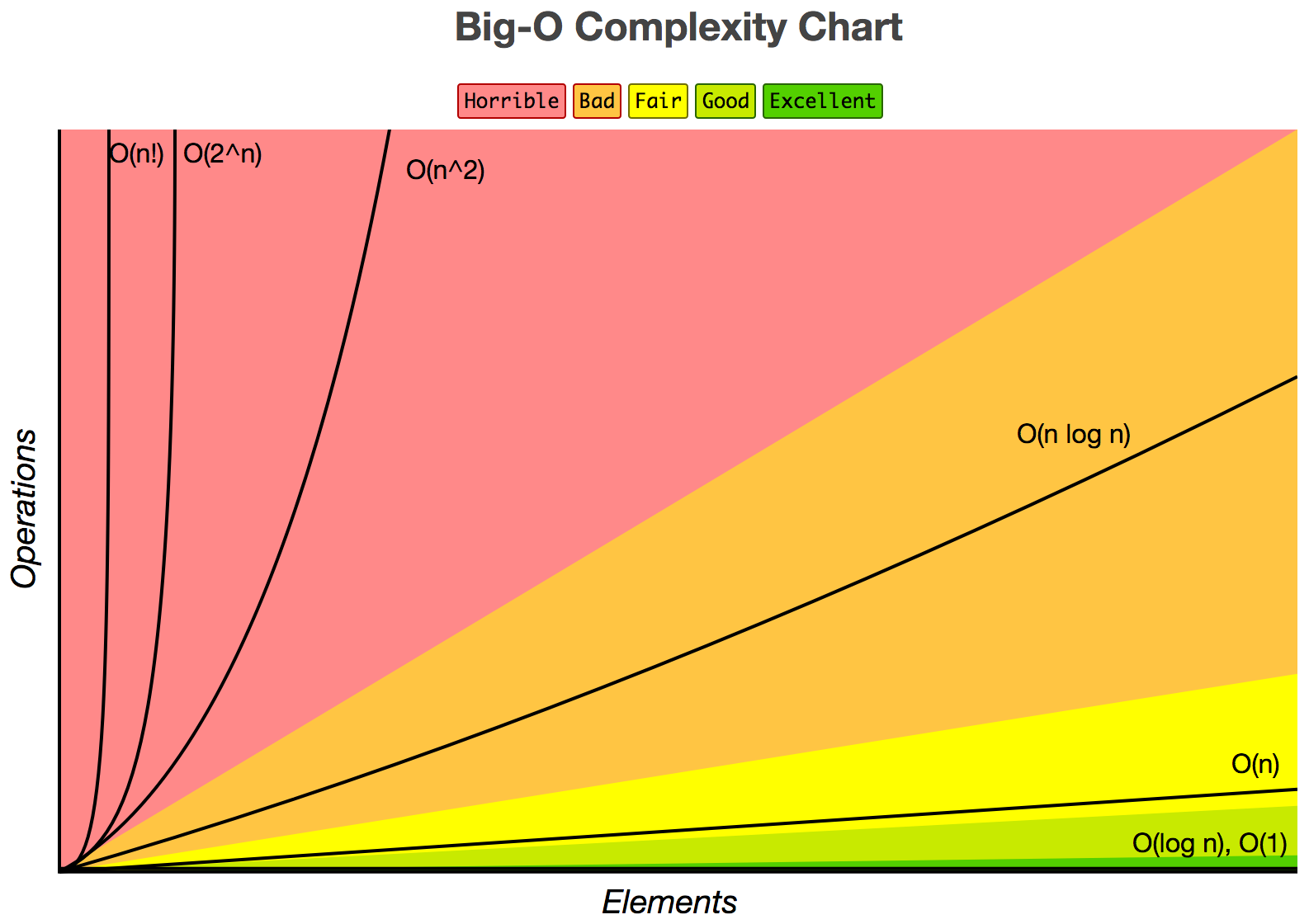
This short video provides a great walkthrough of these curves, giving a simple analogy for their performance.

As the video illustrates, algorithms in the O(1) and O(log n) categories are highly efficient and scalable, while those in O(n²) and beyond can become very slow as the input size grows.

Exploring the Common Complexity Classes

Now, let's examine each of the five key complexity classes in more detail. We'll look at the type of operations that characterize each one and see some conceptual code examples.

1. O(1) — Constant Time

As we touched on previously, an algorithm has a constant time complexity if its execution time is independent of the input size (n). It takes the same number of steps whether the input array has 10 elements or 10 million.

Hallmarks:

• No loops that depend on the input size.
• Direct lookups or simple calculations.

Common Examples:

• Accessing an element in an array with its index (e.g., my_array[5]).
• A simple arithmetic operation (e.g., x = 5 + 3).
• Pushing or popping an element from a stack.

Let's watch a more detailed explanation.

2. O(log n) — Logarithmic Time

This is our first new class, and it's a very powerful one. An algorithm is logarithmic if it reduces the size of the problem by a significant fraction (e.g., by half) with each step.

Imagine looking for a name in a physical phone book. You don't start at the first page and read every name. Instead, you open to the middle. If the name you're looking for comes alphabetically after the names on that page, you discard the entire first half of the book and repeat the process on the second half. This is the core idea of a logarithmic operation.

Hallmarks:

• The algorithm repeatedly divides the input data.
• Often seen in "divide and conquer" approaches on sorted data.

Common Example:

• Binary Search: The classic example of O(log n). It works only on sorted data.

The key takeaway is that for an input of size n, the number of steps is roughly log₂(n). Even if n is a billion, log₂(n) is only about 30. This makes O(log n) algorithms incredibly scalable.

3. O(n) — Linear Time

We've seen this one before. An algorithm has linear time complexity if its runtime grows in direct proportion to the input size. If you double the input, you double the work.

Hallmarks:

• A single loop that iterates through all n elements.

Common Examples:

• Searching for an element in an unsorted array (linear search).
• Finding the maximum or minimum value in an unsorted array.
• Summing all elements in an array.

4. O(n log n) — Linearithmic Time

This complexity class is a common and very important one, especially in sorting. Think of it as a hybrid: it means the algorithm does an O(log n) operation for each of the n elements.

Hallmarks:

• Many efficient "divide and conquer" sorting algorithms fall into this category. They work by breaking the input into smaller pieces, sorting them, and then merging them back together.

Common Examples:

• Merge Sort and Heapsort are classic O(n log n) sorting algorithms. We will implement these later in the course.
• Most general-purpose sorting functions provided by programming languages (like C's qsort) have an average-case complexity of O(n log n).

O(n log n) is slightly less efficient than O(n), but it is dramatically better than O(n²), making it the gold standard for many common problems.

5. O(n²) — Quadratic Time

Finally, quadratic time complexity occurs when the runtime is proportional to the square of the input size. If the input size doubles, the runtime roughly quadruples.

Hallmarks:

• A nested loop where both the inner and outer loops iterate over the n elements.

Common Examples:

• Simple sorting algorithms like Bubble Sort, Selection Sort, and Insertion Sort.
• Finding if there are any duplicate values in a list by comparing every element to every other element.
• Iterating over all pairs of elements in a collection.

This article from GeeksforGeeks provides a good summary of these classes with C-style code snippets.

Quantitative Comparison

Seeing the notations is one thing, but seeing the numbers really drives home the difference in performance. The table below shows the approximate number of operations for each complexity class as the input size n grows.

n	O(log n)	O(n)	O(n log n)	O(n²)
10	~3	10	~33	100
100	~7	100	~664	10,000
1,000	~10	1,000	~9,965	1,000,000
10,000	~13	10,000	~132,877	100,000,000

Table based on data from GeeksforGeeks.

Look at the row for n = 10,000.

• An O(n) algorithm takes 10,000 steps.
• An O(n log n) algorithm takes about 133,000 steps. Manageable.
• An O(n²) algorithm takes 100 million steps. This is where a program that was fast on a small input can slow to a crawl.

This dramatic difference is why understanding Big-O is not just an academic exercise; it's a practical necessity for writing scalable and performant software.

Conclusion

In this lesson, we put the five most common complexity classes under the microscope. By understanding the characteristics of each, you can start to predict an algorithm's performance just by looking at its structure.

Key Takeaways:

• O(1) (Constant): Blazingly fast. The runtime doesn't depend on the input size. Example: array[i].
• O(log n) (Logarithmic): Excellent scalability. The algorithm halves the work at each step. Example: binary search.
• O(n) (Linear): Good, predictable performance. The work scales directly with the input. Example: a single for loop.
• O(n log n) (Linearithmic): Very good. The standard for efficient sorting algorithms. Example: merge sort.
• O(n²) (Quadratic): Becomes slow quickly. Often involves nested loops over the same data. Example: bubble sort.

Preview of the Next Lesson:
Now that you can identify and compare these complexity classes, the next step is to practice applying this knowledge. In the next lesson, we will focus on analyzing simple C code snippets, including single loops, consecutive loops, and nested loops, to determine their Big-O time complexity on your own.