Probability Distributions in ML

Welcome to the start of your journey into the theoretical foundations of machine learning. Given your extensive background in computer science, you're well-equipped to appreciate the rigorous, formal-yet-practical nature of this field. This first module establishes the mathematical bedrock upon which all machine learning is built.

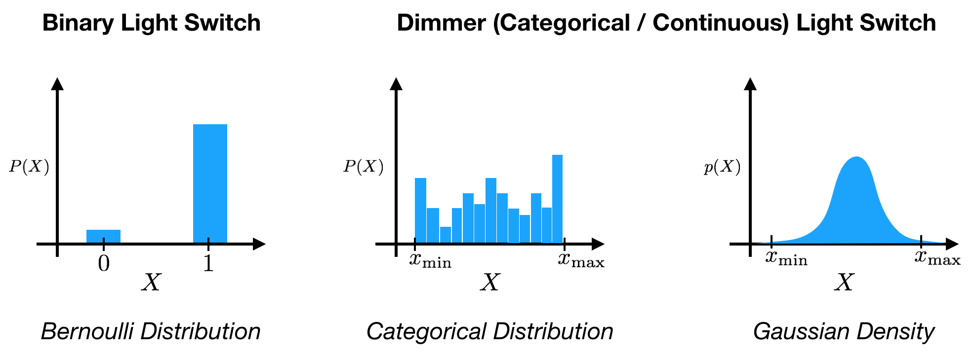
Our first topic is probability distributions. In machine learning, we are almost always dealing with uncertainty—uncertainty in our data, in our model's predictions, and in the parameters of the model itself. Probability distributions provide the mathematical language to quantify and manipulate this uncertainty. In this lesson, we will describe three of the most important distributions—Bernoulli, Categorical, and Gaussian—and explore their fundamental roles in framing and solving machine learning problems. This will lay the groundwork for our next topic: using data to update our beliefs, a core concept in learning.

From Randomness to Real Numbers

At its heart, machine learning is about building models from data. Since data is generated by real-world processes that are inherently random or too complex to model deterministically, we turn to probability.

A random variable, typically denoted by a capital letter like $X$, is a variable whose value is a numerical outcome of a random phenomenon. It provides a crucial bridge from abstract outcomes (like "heads" or "tails") to the real number line, where we can perform mathematical operations.

To begin, let's watch a segment from a Stanford lecture that reviews these foundational concepts.

As the video explains, for a discrete random variable, the PMF, $P(X=x)$, gives the probability that the variable takes on a specific value $x$. The sum of all probabilities across all possible values is 1.

For a continuous random variable, the PDF, $f(x)$, is a function where the area under the curve between two points $a$ and $b$ gives the probability $P(a\le X\le b)$. A key and sometimes counter-intuitive point is that for any continuous random variable, the probability of it taking on any single specific value is zero. Probability is only non-zero over an interval.

Distributions for Classification: Bernoulli and Categorical

Many machine learning problems are classification tasks, where the goal is to assign a label to an input. The Bernoulli and Categorical distributions are the natural starting points for modeling these labels.

The Bernoulli Distribution: Two Possible Outcomes

The simplest case is binary classification, where there are only two possible outcomes.

• Is an email spam or not spam?
• Will a customer click on an ad or not?
• Is a credit card transaction fraudulent or legitimate?

The Bernoulli distribution models a single trial with two outcomes, typically labeled 0 (failure) and 1 (success). It is defined by a single parameter, $p$, which is the probability of the outcome being 1.

The video below provides a concise explanation.

As the video shows, the PMF can be written elegantly as:

$$P(X=x)=p^x(1-p{)}^{1-x}\text{for }x\in \{0,1\}$$

If the outcome $x$ is 1 (success), the $(1-p{)}^{1-1}$ term becomes 1, leaving $p$. If the outcome $x$ is 0 (failure), the $p^0$ term becomes 1, leaving $1-p$.

In machine learning, we don't just model a single event. We build models that predict the parameter $p$ based on some input features. For example, in logistic regression, the model takes the features of an email (words, sender, etc.) and computes a probability $p$ that the email is spam ($y=1$).

The Categorical Distribution: Multiple Possible Outcomes

When a classification task involves more than two outcomes, we generalize from the Bernoulli to the Categorical distribution.

• Classifying a handwritten digit (0, 1, ..., 9).
• Identifying the species of a flower from a photograph.
• Tagging a news article with a topic (e.g., 'Sports', 'Politics', 'Technology').

The Categorical distribution models a single trial with $K$ possible outcomes. It is parameterized by a vector of probabilities $\mathbf{p}=[p_1,p_2,\dots ,p_K]$, where $p_k$ is the probability of the $k$-th outcome, and ${\sum }_{k=1}^K{p}_k=1$.

In an ML context, a multi-class classification model (like a neural network with a softmax output layer) takes an input (e.g., an image) and outputs the parameter vector $\mathbf{p}$, representing the probability for each of the $K$ classes.

To deepen your theoretical understanding, the following reading from Tom Mitchell's book formally introduces these distributions and, importantly, connects them to the fundamental ML concept of parameter estimation.

The Gaussian Distribution: Modeling Continuous Data

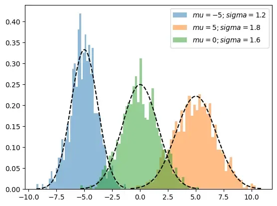
While discrete distributions are perfect for labels, much of the data we encounter in the real world is continuous: sensor readings, financial data, physical measurements, etc. The most important distribution for modeling such data is the Gaussian distribution, also known as the Normal distribution or "bell curve."

It is defined by two parameters:

1. The mean ($\mu$), which represents the center or expected value of the distribution.
2. The variance (${\sigma }^2$), which measures the spread or dispersion of the data around the mean. The square root of the variance, $\sigma$, is the standard deviation.

The PDF of the Gaussian distribution is:

$$f(x|\mu ,{\sigma }^2)=\frac{1}{\sqrt{2\pi {\sigma }^2}}\exp \left(-\frac{(x-\mu {)}^2}{2{\sigma }^2}\right)$$

Let's consult the Stanford course notes for a formal description.

The Gaussian distribution is ubiquitous in machine learning for several reasons:

• Modeling Features: It's often a reasonable assumption for the distribution of real-valued input features, such as the height of a person or the price of a stock.
• Modeling Noise: In regression problems, we often assume that the errors (the difference between our model's predictions and the true values) are Gaussian-distributed. This assumption is the foundation for models like linear regression.
• Central Limit Theorem: This powerful theorem states that the sum of many independent random variables tends toward a Gaussian distribution, regardless of the original distributions. This provides a theoretical justification for its widespread appearance.
• Mathematical Convenience: The Gaussian has mathematical properties that make it easy to work with in many derivations.

The Multivariate Gaussian Distribution

In practice, our data rarely consists of a single feature. We usually work with data points that are vectors in a high-dimensional space (e.g., an image is a vector of pixel values). The Multivariate Gaussian distribution is the generalization of the Gaussian to multiple dimensions.

Instead of a scalar mean $\mu$ and variance ${\sigma }^2$, it is parameterized by:

• A mean vector $\mathbf{\mu }$, which defines the center of the distribution in $n$-dimensional space.
• A covariance matrix $\mathbf{\Sigma }$, an $n\times n$ matrix that describes not only the variance of each dimension along its diagonal but also how the dimensions vary with respect to each other (the covariance) in its off-diagonal elements.

The Stanford lecture video provides excellent visual intuition for how $\mathbf{\mu }$ and $\mathbf{\Sigma }$ shape the distribution.

Conclusion

In this introductory lesson, we have established the first pillar of our theoretical foundation. We explored how random variables and probability distributions are used to formally describe data-generating processes.

Here are the key takeaways:

• Probability distributions are the language of uncertainty in machine learning. We distinguish between discrete variables (modeled by PMFs) and continuous variables (modeled by PDFs).
• The Bernoulli distribution models a single trial with two outcomes and is the foundation for binary classification. It is parameterized by $p$, the probability of success.
• The Categorical distribution generalizes the Bernoulli to a single trial with $K$ outcomes, making it the basis for multi-class classification. It is parameterized by a vector of $K$ probabilities.
• The Gaussian distribution is the most common model for continuous data, defined by its mean $\mu$ and variance ${\sigma }^2$. Its multivariate version is critical for modeling high-dimensional data vectors, using a mean vector $\mathbf{\mu }$ and a covariance matrix $\mathbf{\Sigma }$.

In our next lesson, we will build directly on these concepts. Now that we can postulate a probabilistic model for our data, we will ask: how can we use observed data to infer the parameters of our model? This will lead us to one of the most fundamental rules in all of statistics and machine learning: Bayes' theorem.