Recommended resources
The freely available resources this lesson will direct you to.

Hello! This first module begins with the big picture: what data engineers move, where they move it, and who uses the result. Later lessons will give you the tools to build each part. For now, you will follow one batch pipeline from e-commerce source systems to a sales dashboard. By the end, you should be able to explain not just the stages, but what happens to a particular record at each stage.
What makes a pipeline a pipeline?
An online shop records purchases so it can take payments and fulfill orders. A sales team asks a different question: “How much revenue did each product category generate yesterday?” Answering that question repeatedly requires data to be collected, prepared, stored for analysis, and made available to a report. A data pipeline is the repeatable process that does this work.
Begin with Chandoo’s What is ETL with a clear example. The opening explains why repeatedly preparing a report by hand is costly; the later example shows how detailed sales records become a summary.
What is ETL with a clear example - Data Engineering Concepts
Watch Chandoo’s “What is ETL with a clear example” to see the purpose of extract, transform, and load in a recurring reporting task.
Watch the ETL introduction, then skip to the sales example. In the example, distinguish the detailed records needed to handle an individual delivery from the monthly totals needed for reporting. You do not need to learn the SQL shown later in the video.
ETL names one common pipeline pattern: extract data from a source, transform it into a useful form, then load it into a destination. The source might be a database, an application interface, or a file. Transforming can mean correcting formats, excluding records that do not qualify for a report, combining sources, or calculating totals. Loading means writing the prepared result somewhere an analytics consumer can access it.
A pipeline is the broader idea; ETL is one way to arrange its work. Not every pipeline transforms data before loading it into its final processing environment. What matters for this lesson is that you can identify where a record came from, what happened to it, where the result went, and who uses it.
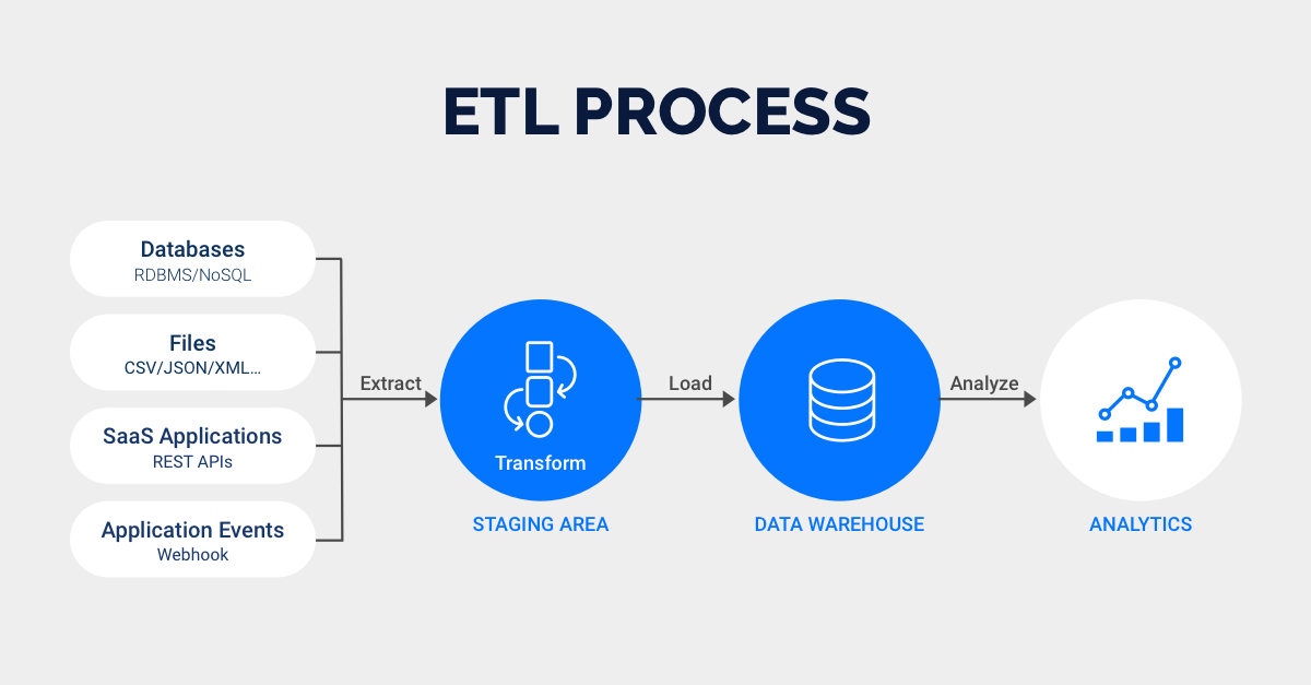
The diagram calls the temporary working area staging. Think of it as a place where a run can prepare data before the analytical destination is updated, not as the final report. The data warehouse is the destination shown here for prepared analytical data. The analytics consumer is the report, dashboard, analyst, or other system that reads the result. A warehouse may hold detailed records as well as summaries; the diagram does not require every pipeline to aggregate.
What changes when the pipeline runs in batches?
A batch pipeline handles a defined collection of records on a run, often according to a schedule. A nightly sales run might process purchases from the preceding calendar day. It does not update the dashboard at the instant each customer checks out.
Read the Batch processing pipelines section of IBM’s What Is a Data Pipeline? for the relationship between scheduled runs and their successive processing steps.
Read IBM’s “What Is a Data Pipeline?” to establish what a scheduled batch run does and why its steps must fit together.
In “Batch processing pipelines,” begin with the paragraph opening “As the name implies, batch processing loads.” Read the batch explanation through the paragraph ending “written to the repository.” Focus on the distinction between a scheduled collection of data and the successive jobs that prepare and write it; the earlier history of batch processing is not needed here.
Two pieces of time are worth keeping separate:
- The data window specifies which source records belong to the run—for example, purchases made on June 3.
- The run time is when the pipeline processes that window—for example, 01:00 on June 4.
If the run completes at 01:10, a dashboard using its output can report on June 3 purchases. It should not claim to show every purchase made up to 01:10 on June 4. This difference between when business activity happened and when analysis became available is called data freshness.
Scheduling alone does not guarantee a correct result. The extraction must select the intended records, the transformations must apply the intended business rules, and the load must complete before the consumer reads the new result.
Follow a purchase all the way to a dashboard
Suppose an e-commerce team wants a daily report of paid-order revenue by product category. An operational orders database holds individual purchases, while a product file identifies each product’s category. To keep the example focused, each order has one product and one amount, expressed in INR.
For the June 3 data window, the orders database contains:
| Order ID | Product | Status | Amount |
|---|---|---|---|
| 1042 | P7 | Paid | 1,200 |
| 1043 | P8 | Paid | 800 |
| 1044 | P7 | Cancelled | 500 |
The product file says that both P7 and P8 belong to the Home category. The intended report should therefore show two paid orders and 2,000 INR in revenue for Home. The cancelled order must not contribute.
At the sources, order 1042 exists because the shop recorded a purchase. The product file has a separate purpose: describing products. Neither source is itself the daily category report. A source system is where data originates for this pipeline, even if that system also serves other purposes.
During extraction, the nightly run reads the orders belonging to June 3 and the product information it needs. Imagine that a retry causes order 1042 to appear twice in the extracted input. There are now four extracted order rows, although the source example contains only three distinct orders. Extraction has brought data into the pipeline; it has not yet made that data safe to total.
Some pipelines retain an unchanged copy of extracted records in a raw-data area. This gives engineers evidence of what arrived and a starting point if a transformation needs to be rerun. A raw copy is not the same as the finished analytical result. The illustrated ETL diagram does not show this optional area, but you will encounter it in later pipeline designs.
During transformation, the run removes the extra copy of order 1042, excludes cancelled order 1044 under the report’s business rule, and uses the product file to assign a category to orders 1042 and 1043. It can then calculate the Home total: two qualifying orders with amounts of 1,200 and 800 INR. Notice that “cleaning” is not merely changing how values look. Choosing which orders count is a decision about the meaning of the metric.
During loading, the run writes the prepared result to an analytical table in the warehouse. For this example, one resulting row could contain the reporting date June 3, category Home, paid-order count 2, and revenue 2,000 INR. That row summarizes the qualifying orders; it is not a replacement for the individual purchase records in the operational system.
At consumption, a dashboard reads the warehouse result and displays the category total. The dashboard is an analytics consumer, not the source of the purchase data. If it caches results, it may also need to refresh before viewers see the newly loaded figures.
You can now trace order 1042 in words: it was recorded as a paid purchase, included in the June 3 extraction, retained once despite the duplicate extracted copy, classified as Home using the product file, included in the warehouse’s Home total, and represented in the dashboard figure. You cannot recover all of order 1042’s details from the summary row alone. To investigate the individual contribution, you also need the source or retained raw records and knowledge of the transformation rules.
A successful run is more than a completed load
Suppose the dashboard displays 2,500 INR for Home. The difference from the expected 2,000 INR gives you a useful path of investigation. Did the extraction include an unintended order? Did transformation incorrectly include cancelled order 1044? Was order 1042 counted twice? Or is the dashboard showing a different reporting date? Tracing the result means checking each stage against the question the report was meant to answer.
Simple run records make that possible. For this example, an engineer might record the selected date window, the number of extracted rows, the number of distinct orders, the number excluded by the paid-only rule, whether the warehouse load completed, and when the consumer last refreshed. Those facts do not prove that every business rule is right, but they help locate where an unexpected number arose.
A failed load has a different consequence from a bad calculation. If the warehouse was not updated, the dashboard may still show yesterday’s successfully loaded result rather than an obviously broken page. A report therefore needs an understandable “as of” time as well as a value. Late changes to source records can also affect a date that was previously reported; later in the course, you will learn ways to update such results reliably.
Key takeaways
A batch pipeline processes a defined set of source data on a run. In the ETL pattern, it extracts records, transforms them according to the analytical need, and loads the prepared result for a consumer. To trace data well, follow both an individual record and the reported value it contributes to, while keeping the data window, run time, and report freshness distinct.
The next lesson looks more closely at the storage roles mentioned here: transactional databases, analytical warehouses, and data lakes.