Dyson's Equation for the Single-Particle Green's Function

Hello! Welcome back to our journey into diagrammatic many-body theory.

In our last lesson, we discovered how to translate the abstract perturbation series for the Green's function into a concrete set of pictures—Feynman diagrams. We learned the rules for drawing these diagrams and translating them back into mathematical expressions. However, calculating the Green's function by summing diagrams one by one is an infinite task.

Today, we will take a monumental step forward. We'll learn how to tame this infinite series by grouping diagrams in a clever way. This will lead us to one of the most powerful and central results in many-body physics: Dyson's equation. This equation provides a compact, non-perturbative expression for the exact Green's function, $G$, by introducing a new, crucial object: the self-energy, $\Sigma$. You will learn not just one, but two distinct ways to derive this equation, giving you a deep and flexible understanding of its origin and meaning.

1. From Infinite Series to a Closed Equation

The key idea is to organize the infinite sum of diagrams not by the number of interactions, but by their topology. This allows us to sum infinite sub-classes of diagrams at once.

Irreducible Diagrams and the Self-Energy

Let's classify the connected diagrams that contribute to the full propagator $G$.

• A diagram is reducible if it can be split into two disconnected pieces by cutting a single internal free propagator line ($G_0$).
• A diagram is irreducible (or, more precisely, one-particle irreducible) if it is connected and cannot be split in this way.

Examples of reducible and irreducible diagrams. The reducible diagram can be cut along the dashed line (a single G_0 line) to fall into two pieces. The irreducible diagrams cannot.

We now define the proper self-energy, ${\Sigma }^{\star }(k,\omega )$, as the sum of all possible irreducible diagrams with one incoming and one outgoing line, but with the two external propagator legs "amputated" (removed).

The video below will walk you through this classification and show how it leads directly to Dyson's equation.

Dyson's Equation

As you saw in the video, the entire infinite series of diagrams for the full propagator $G$ can be summed up into a beautifully simple diagrammatic equation:

.

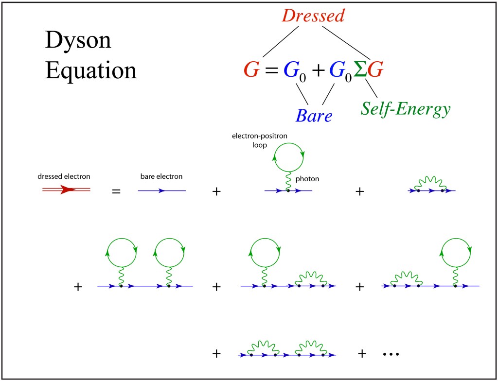
Translating this picture into mathematics (in momentum-frequency space) gives us Dyson's equation:

$$G(k,\omega )=G_0(k,\omega )+G_0(k,\omega ){\Sigma }^{\star }(k,\omega )G(k,\omega )$$

This is an algebraic equation for $G(k,\omega )$ which we can easily solve. Rearranging the terms, we get:

$$G(k,\omega )[1-G_0(k,\omega ){\Sigma }^{\star }(k,\omega )]=G_0(k,\omega )$$ $$G(k,\omega )=\frac{G_0(k,\omega )}{1-G_0(k,\omega ){\Sigma }^{\star }(k,\omega )}$$

Recalling that the free propagator is $G_0(k,\omega )=(\omega -{ϵ}_k+i\delta {)}^{-1}$ (we'll set $\hslash =1$), we can write $G_0^{-1}=\omega -{ϵ}_k$. Substituting this into the denominator gives the most common and insightful form of Dyson's equation:

$$G(k,\omega )=\frac{1}{G_0(k,\omega {)}^{-1}-{\Sigma }^{\star }(k,\omega )}=\frac{1}{\omega -{ϵ}_k-{\Sigma }^{\star }(k,\omega )}$$

This is a profound result. We have replaced an infinite sum of diagrams with a single, compact expression. The entire complexity of the many-body interactions is now encapsulated in one function: the self-energy ${\Sigma }^{\star }(k,\omega )$.

2. Physical Interpretation of the Self-Energy

Dyson's equation is not just a mathematical convenience; it gives us deep physical insight. By comparing the form of the full propagator $G$ with the free one $G_0$, we see that the bare particle's energy ${ϵ}_k$ has been replaced by a complex, energy-dependent quantity ${ϵ}_k+{\Sigma }^{\star }(k,\omega )$. The self-energy literally describes how the energy of the particle is modified by its interactions with the surrounding medium.

The self-energy is a complex function, and its real and imaginary parts have distinct physical meanings.

$${\Sigma }^{\star }(k,\omega )=\text{Re}[{\Sigma }^{\star }(k,\omega )]+i\text{Im}[{\Sigma }^{\star }(k,\omega )]$$

Substituting this into the expression for $G$:

$$G(k,\omega )=\frac{1}{\omega -({ϵ}_k+\text{Re}[{\Sigma }^{\star }])-i\text{Im}[{\Sigma }^{\star }]}$$

1. Real Part $\text{Re}[{\Sigma }^{\star }]$: Energy Renormalization. The real part of the self-energy shifts the energy of the particle. The new, "renormalized" energy of the excitation is no longer ${ϵ}_k$, but a solution to ${\widetilde{ϵ}}_k={ϵ}_k+\text{Re}[{\Sigma }^{\star }(k,{\widetilde{ϵ}}_k)]$. This shift can lead to concepts like the effective mass of a particle in a medium. This "dressed" particle, which incorporates the cloud of interactions surrounding it, is what we call a quasiparticle.

2. Imaginary Part $\text{Im}[{\Sigma }^{\star }]$: Finite Lifetime. In our previous work, the poles of the Green's function were on the real axis. Now, the pole is shifted into the complex plane by $i\text{Im}[{\Sigma }^{\star }]$. A complex pole in energy corresponds to an exponential decay in time. This means the quasiparticle is no longer a stable eigenstate but has a finite lifetime, $\tau$. The lifetime is inversely proportional to the imaginary part of the self-energy: $\tau \propto 1/|\text{Im}[{\Sigma }^{\star }]|$. The imaginary part represents the rate of scattering processes that can destroy the quasiparticle state.

Test your understanding!

A theorist calculates the self-energy for a quasiparticle near the Fermi surface and finds that $\text{Im}[\Sigma^\star(k, \omega)] \to 0$ as $\omega \to E_F$ and $|k| \to k_F$. What is the physical implication of this result?

Show answer

The imaginary part of the self-energy determines the quasiparticle's decay rate (lifetime $\tau \propto 1/|\text{Im}[\Sigma^\star]|$). The fact that $\text{Im}[\Sigma^\star]$ goes to zero at the Fermi surface implies that the lifetime of these quasiparticles becomes infinite. This means that low-energy excitations right at the Fermi surface are stable and well-defined, which is the foundational concept of Landau's Fermi liquid theory.

3. An Alternative View: The Equation of Motion Method

The diagrammatic approach is intuitive and powerful, but there is another way to derive Dyson's equation that does not rely on diagrams at all: the equation of motion (EOM) method. This technique leverages the Heisenberg equation of motion for operators and is a cornerstone of many-body theory in its own right. Given your background, seeing this alternative derivation will provide a more robust understanding.

The basic strategy is:

1. Start with the definition of the Green's function: $G_{AB}(t-t^{\prime })=-i\Theta (t-t^{\prime })⟨[A(t),B(t^{\prime }){]}_{\pm }⟩$.
2. Take its time derivative, $\frac{d}{dt}{G}_{AB}(t-t^{\prime })$.
3. Use the Heisenberg equation of motion, $i\frac{dO}{dt}=[O,H]$, to replace the time derivative of the operator $A(t)$.
4. This will relate the Green's function $G_{AB}$ to a new, more complex Green's function involving the commutator $[A,H]$.
5. This process creates a hierarchy of coupled equations. The "art" of the EOM method lies in finding a suitable approximation to truncate this hierarchy.

The following video provides a masterful demonstration of this technique applied to the resonant level model, a paradigmatic model in condensed matter physics describing a single quantum level coupled to a continuum of states (a "bath").

In the video's final result for the level Green's function $G_L(\omega )$, you saw an expression of the form:

$$G_L(\omega )=\frac{1}{\omega -{ϵ}_0-{\sum }_k\frac{|t_k{|}^2}{\omega -{ϵ}_k+i\delta }}$$

Compare this to the general form of Dyson's equation we found:

$$G(\omega )=\frac{1}{\omega -{ϵ}_0-{\Sigma }^{\star }(\omega )}$$

It's a perfect match! The EOM calculation has automatically generated the self-energy for the resonant level:

$${\Sigma }^{\star }(\omega )=\sum _k\frac{|t_k{|}^2}{\omega -{ϵ}_k+i\delta }$$

This self-energy physically represents the influence of the entire bath of states (indexed by $k$) on the single level ${ϵ}_0$. The particle can "hop" from the level into the bath and back, and the self-energy captures the net effect of all these virtual processes. This provides a powerful, non-diagrammatic way to understand and calculate the self-energy.

Conclusion

Today we have reached a major milestone. We have tamed the infinite perturbative expansion for the Green's function and condensed it into the elegant and powerful Dyson's equation.

Key Takeaways:

• The full Green's function $G$ can be expressed in terms of the free Green's function $G_0$ and the proper self-energy ${\Sigma }^{\star }$.
• Dyson's equation provides this connection: $G(k,\omega )=(\omega -{ϵ}_k-{\Sigma }^{\star }(k,\omega ){)}^{-1}$.
• The self-energy ${\Sigma }^{\star }$ is the sum of all one-particle irreducible diagrams and represents the total effect of interactions on a propagating particle.
• The real part of ${\Sigma }^{\star }$ renormalizes the particle's energy, while its imaginary part gives the particle a finite lifetime.
• The Equation of Motion (EOM) method provides an alternative, non-diagrammatic route to deriving Green's functions and identifying the self-energy.

Preview of the Next Lesson:

Dyson's equation shifts the central problem of many-body theory from calculating $G$ to calculating ${\Sigma }^{\star }$. The entire game is now to find good approximations for the self-energy. In our next lesson, we will apply this new framework to a cornerstone model of condensed matter physics: the Jellium model for the interacting electron gas. We will calculate the self-energy in the first-order (Hartree-Fock) approximation, re-deriving our result from the previous lesson but now from the more powerful perspective of the self-energy.