Diffusion Models: Forward Corruption and Learned Reverse Processes

Hello, and welcome to the first lesson in Diffusion Models in ML. This first module builds the basic construction that everything else in the course relies on: a known process that progressively corrupts data, and a learned process that turns noise back into data.

By the end of this lesson, you should be able to write down both probability models, explain why one is fixed while the other must be learned, and describe exactly what happens when a diffusion model generates an image. We will intentionally postpone the training-loss derivation: the immediate task is to understand the two chains and their roles.

---

The central idea: make generation a sequence of manageable denoising decisions

A generative model should produce new samples that resemble the training data: for example, plausible faces, molecules, audio clips, or images. Diffusion models do this by beginning with a simple distribution we can sample from easily, usually standard Gaussian noise, and transforming it into data through many small stochastic denoising steps.

The construction is easiest to understand in the opposite direction first:

1. Take a real data example ${\mathbf{x}}_0$, such as a clean image.
2. Add a small amount of random Gaussian noise.
3. Repeat the corruption many times until the result ${\mathbf{x}}_T$ is nearly indistinguishable from Gaussian noise.
4. Learn to run a corresponding process in reverse, moving from ${\mathbf{x}}_T$ back toward a clean sample.

The key asymmetry is deliberate:

• Forward corruption is designed by us and entirely known.
• Reverse denoising depends on the unknown data distribution, so its transitions must be learned from examples.

Watch the following short segments from Ari Seff’s What are Diffusion Models? for a visual first pass through this construction.

A Markov chain is central here. It means the next state depends on the present state, rather than needing the complete past history. For the forward chain, once ${\mathbf{x}}_{t-1}$ is known, the earlier states ${\mathbf{x}}_0,\dots ,{\mathbf{x}}_{t-2}$ are irrelevant for producing ${\mathbf{x}}_t$.

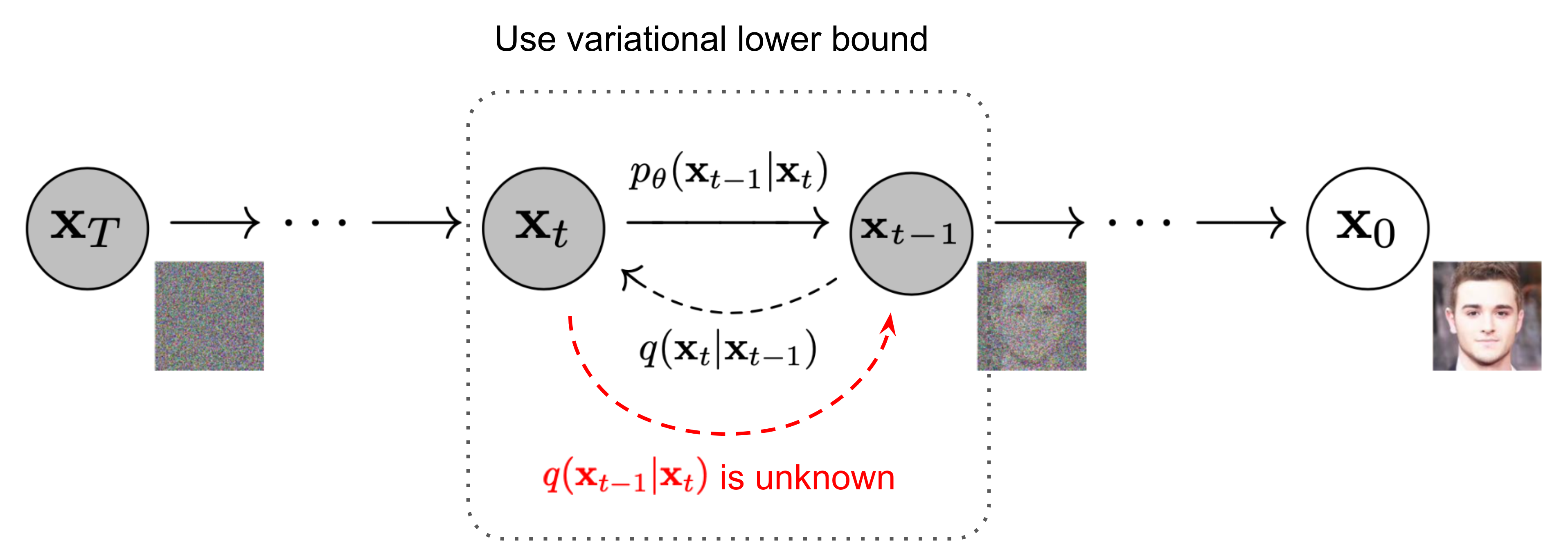
The figure is laid out with clean data on the right and noise on the left, so its visual direction is opposite the usual timestep order. Mathematically, the forward process still runs from $t=0$ to $t=T$; sampling runs from $t=T$ down to $t=0$.

---

The fixed forward diffusion process

Let ${\mathbf{x}}_0$ denote a data vector. For an RGB image, it might have shape $H\times W\times 3$, but the mathematics treats it as one high-dimensional vector. Diffusion creates noisy versions

$${\mathbf{x}}_1,{\mathbf{x}}_2,\dots ,{\mathbf{x}}_T.$$

Choose a variance schedule:

$${\beta }_1,{\beta }_2,\dots ,{\beta }_T,$$

where each ${\beta }_t$ is small and positive. The schedule specifies how much fresh noise is injected at each step. Define

$${\alpha }_t=1-{\beta }_t.$$

The one-step forward transition is a Gaussian:

$$q({\mathbf{x}}_t\mid {\mathbf{x}}_{t-1})=\mathcal{N}\left({\mathbf{x}}_t;\sqrt{{\alpha }_t}{\mathbf{x}}_{t-1},{\beta }_t\mathbf{I}\right).$$

Equivalently, we can sample this transition as

$${\mathbf{x}}_t=\sqrt{{\alpha }_t}{\mathbf{x}}_{t-1}+\sqrt{{\beta }_t}{\mathbf{ϵ}}_t,{\mathbf{ϵ}}_t\sim \mathcal{N}(0,\mathbf{I}).$$

Each step has two effects:

• It slightly shrinks the previous sample by $\sqrt{{\alpha }_t}$.
• It adds independent Gaussian noise with variance ${\beta }_t$.

The full forward chain is therefore

$$q({\mathbf{x}}_{1:T}\mid {\mathbf{x}}_0)=\prod _{t=1}^{T}q({\mathbf{x}}_t\mid {\mathbf{x}}_{t-1}).$$

This is called fixed because it contains no learned parameters $\theta$. Once you select $T$ and the schedule $\{{\beta }_t\}$, you can generate a noisy version of any training image immediately.

A subtle but important point: the forward process is not a generator. It does not learn, identify objects, or create new semantic content. Its job is to convert a complicated data distribution into a simple terminal distribution that is approximately

$${\mathbf{x}}_T\sim \mathcal{N}(0,\mathbf{I}).$$

The ability to sample standard Gaussian noise is what makes the eventual generative procedure practical.

Read the two opening subsections of Lilian Weng’s What are Diffusion Models? to reinforce the formal definition and see the forward and reverse chains placed side by side.

It is common to use $q$ for both the data-associated forward process and related distributions. Keep the roles straight:

• $q({\mathbf{x}}_t\mid {\mathbf{x}}_{t-1})$ is the chosen corruption rule.
• $q({\mathbf{x}}_{t-1}\mid {\mathbf{x}}_t)$ is the true reverse conditional induced by the data distribution and corruption rule.
• $p_{\theta }({\mathbf{x}}_{t-1}\mid {\mathbf{x}}_t)$ is the learned approximation used at generation time.

---

Why reversing the process is difficult

It may seem that we could simply “subtract the noise” at each step. But the noisy observation ${\mathbf{x}}_t$ generally does not tell us which exact clean image produced it.

Imagine that a heavily corrupted image contains a vague light-colored oval in the center. It might have come from a face, an animal, a bowl, or merely an abstract image. The correct reverse distribution must represent what is plausible under the training data, not just remove pixelwise noise.

Formally, the object we would like to know is

$$q({\mathbf{x}}_{t-1}\mid {\mathbf{x}}_t).$$

Bayes’ rule suggests that it depends on

$$q({\mathbf{x}}_{t-1}\mid {\mathbf{x}}_t)=\frac{q({\mathbf{x}}_t\mid {\mathbf{x}}_{t-1})q({\mathbf{x}}_{t-1})}{q({\mathbf{x}}_t)}.$$

The transition $q({\mathbf{x}}_t\mid {\mathbf{x}}_{t-1})$ is known, because we designed it. The problem lies in the marginal distributions $q({\mathbf{x}}_{t-1})$ and $q({\mathbf{x}}_t)$: they reflect the full, complex distribution of real images after noise has been added. We only have a finite dataset of samples from that distribution, not a simple analytical expression for it.

There is a related conditional distribution,

$$q({\mathbf{x}}_{t-1}\mid {\mathbf{x}}_t,{\mathbf{x}}_0),$$

that becomes tractable because it is allowed to use the original clean sample ${\mathbf{x}}_0$. During training, that clean image is available. During generation, it is exactly what we do not have. The next module will derive this useful training-time posterior carefully.

For now, the essential conclusion is: knowing how to corrupt data does not automatically give us a usable reverse process. We must learn one.

---

The learned reverse Markov chain

Diffusion models define a parameterized reverse-time probability model:

$$p_{\theta }({\mathbf{x}}_{0:T})=p({\mathbf{x}}_T)\prod _{t=1}^T{p}_{\theta }({\mathbf{x}}_{t-1}\mid {\mathbf{x}}_t).$$

Its initial distribution is simple:

$$p({\mathbf{x}}_T)=\mathcal{N}(0,\mathbf{I}).$$

For a standard DDPM, each learned reverse transition is modeled as a Gaussian:

$$p_{\theta }({\mathbf{x}}_{t-1}\mid {\mathbf{x}}_t)=\mathcal{N}\left({\mathbf{x}}_{t-1};{\mathbf{\mu }}_{\theta }({\mathbf{x}}_t,t),{\mathbf{\Sigma }}_{\theta }({\mathbf{x}}_t,t)\right).$$

Here, $\theta$ denotes the parameters of a neural network, typically a U-Net for images. Given a noisy image ${\mathbf{x}}_t$ and a timestep $t$, the network outputs information that determines a distribution for the slightly cleaner sample ${\mathbf{x}}_{t-1}$.

The timestep is necessary. A pattern that looks like weak texture at an early timestep may be mostly random noise at a late timestep. The model needs to know the noise level in order to apply the appropriate denoising behavior.

Component	Forward process $q$	Reverse process $p_{\theta }$
Purpose	Corrupt real data	Generate or denoise samples
Direction in timestep	$0$ through $T$	$T$ down through $0$
Parameters	Fixed schedule $\{{\beta }_t\}$	Learned network parameters $\theta$
Starting point	A real datum ${\mathbf{x}}_0$	Gaussian noise ${\mathbf{x}}_T$
One-step rule	Known Gaussian	Learned Gaussian approximation
Used during generation?	No	Yes

Why use a Gaussian for the reverse step if images are highly complex? The full image distribution is indeed complex and can be multimodal. But the model does not try to transform noise into an image in one Gaussian step. Instead, it composes many small, time-conditioned transitions. A simple local conditional at each step can produce a highly non-Gaussian distribution over final images.

Small forward noise steps also make this modeling choice more reasonable: locally, reversing a tiny Gaussian perturbation can be well approximated by a Gaussian transition whose mean depends on the current noisy sample and the noise level.

---

Sampling: how a new image is generated

After training, generation follows the learned reverse chain.

1. Draw an initial noise tensor:

   $${\mathbf{x}}_T\sim \mathcal{N}(0,\mathbf{I}).$$

2. At timestep $t=T$, feed ${\mathbf{x}}_T$ and $t$ to the denoising network.

3. Use its output to define and sample from

   $$p_{\theta }({\mathbf{x}}_{T-1}\mid {\mathbf{x}}_T).$$

4. Repeat at $t=T-1,T-2,\dots ,1$, each time obtaining a somewhat cleaner sample.

5. Return ${\mathbf{x}}_0$ as the generated image.

The word sample matters. The reverse chain defines distributions, not merely a deterministic editing procedure. Reverse-time randomness allows the model to represent variation among plausible outputs. Later, we will see samplers that intentionally reduce or remove some of this randomness for speed.

At training time, the direction is different:

1. Draw a clean training sample ${\mathbf{x}}_0$.
2. Corrupt it with the fixed forward process to obtain a noisy ${\mathbf{x}}_t$.
3. Adjust $\theta$ so that the learned reverse transition is consistent with how the forward process created that noisy sample.

The precise objective used to make “consistent” mathematically meaningful is the variational diffusion objective, which begins in the next module.

---

A compact formulation checklist

A correct formulation of a basic discrete diffusion generative model should include all five items below:

1. Data variable: ${\mathbf{x}}_0$ is a sample from the unknown data distribution.

2. Forward Markov chain:

   $$q({\mathbf{x}}_{1:T}\mid {\mathbf{x}}_0)=\prod _{t=1}^T\mathcal{N}\left({\mathbf{x}}_t;\sqrt{1-{\beta }_t}{\mathbf{x}}_{t-1},{\beta }_t\mathbf{I}\right).$$

3. Known noise schedule: $\{{\beta }_t{\}}_{t=1}^T$ is fixed before training in the basic DDPM construction.

4. Reverse Markov chain:

   $$p_{\theta }({\mathbf{x}}_{0:T})=\mathcal{N}({\mathbf{x}}_T;0,\mathbf{I})\prod _{t=1}^T{p}_{\theta }({\mathbf{x}}_{t-1}\mid {\mathbf{x}}_t).$$

5. Learned reverse conditional:

   $$p_{\theta }({\mathbf{x}}_{t-1}\mid {\mathbf{x}}_t)=\mathcal{N}\left({\mathbf{x}}_{t-1};{\mathbf{\mu }}_{\theta }({\mathbf{x}}_t,t),{\mathbf{\Sigma }}_{\theta }({\mathbf{x}}_t,t)\right).$$

The forward chain gives the training problem its structure; the learned reverse chain is the actual generative model.

---

Key takeaways

A diffusion model pairs two Markov chains over variables of the same dimensionality as the data:

• The forward process is a fixed, known Gaussian corruption process governed by a noise schedule.
• Repeated forward corruption transforms structured data into a distribution close to standard Gaussian noise.
• The true unconditional reverse conditional depends on the unknown data distribution and cannot be directly computed from the forward transition alone.
• A neural network parameterizes a learned reverse Markov chain, usually with Gaussian transitions conditioned on the noisy sample and timestep.
• Generation begins from Gaussian noise and samples repeatedly from learned reverse transitions until it reaches ${\mathbf{x}}_0$.

Next, we will derive a crucial shortcut: the closed-form distribution of ${\mathbf{x}}_t$ conditioned directly on ${\mathbf{x}}_0$. That result makes it possible to add the appropriate amount of noise at any timestep without simulating every preceding forward step.