Unit-Cost Modeling for Training and Inferencecuntegn

Hello! Last lesson separated the services that decide what should run from the workers and serving replicas that do the work. That distinction matters financially: a training job consumes accelerator time and moves data, while shared schedulers and registries also cost money even though they do not execute the model.

This lesson turns those resource estimates into unit-cost models. You’ll build one for a completed training job and one for a successful inference request, then test how pricing, utilization, and performance requirements change the answer. The figures below are illustrative assumptions, not current provider prices. Allow about 40 minutes for the readings, video, and worked models.

---

Start with the unit and the accounting boundary

“Cost per model” and “cost per request” sound precise, but neither is useful until you define what counts.

For training, a practical unit is one successfully delivered training run: a run that produces the specified artifact and passes its required checks. Its boundary might include compute, retries, data access, checkpoints, and a share of platform services. If data preparation or evaluation happens in separate jobs, record those separately or deliberately include them. Do not silently omit them in one comparison and include them in another.

For serving, a practical unit is one successful inference request over a stated period and workload mix. You need both the period’s total cost and its count of successful requests:

$$\text{Cost per successful request}=\frac{\text{serving cost during the period}}{\text{successful requests during the period}}.$$

Failures and retries require care. They can consume resources without increasing the denominator. Likewise, a provisioned accelerator costs money while it is ready but idle; its bill does not shrink just because utilization does.

The FinOps for AI Overview distinguishes usage-based, committed, provisioned, and interruptible pricing. Read its pricing table alongside its unit-cost definitions. Its “training cost efficiency” metric divides cost by a performance score; that can be a supplementary comparison, but it is not a substitute for an itemized cost per completed run.

A useful cost ledger has three columns: quantity, rate, and extended cost. For example, accelerator-hours are a quantity; currency per accelerator-hour is a rate. Keep observed workload quantities separate from quoted prices so that you can update a rate without rebuilding the workload estimate.

The ledger also needs an allocation rule for shared services. If a registry, scheduler, or monitoring stack supports many workloads, you might allocate its monthly cost by reserved capacity, accelerator-hours, request volume, or another documented driver. No rule is perfect; consistency and visibility are more valuable than hiding shared cost inside an unexplained percentage. The data-plane/control-plane boundary from last lesson helps identify these costs, but both planes belong in a full service-cost view.

---

Build the training-job model

Return to the representative four-accelerator job from the earlier capacity estimate. Suppose a successful attempt runs for eight hours. For this example, accelerator and host capacity are billed separately; on an actual bundled instance, use the whole instance price once rather than adding a second host charge.

Input for one delivered run	Illustrative assumption	Cost
Accelerator capacity	4 accelerators × 8 hours × $3 per accelerator-hour	$96
Separately billed host capacity	8 hours × $1.50 per hour	$12
Expected extra billed compute from restarts	10% of the $108 compute subtotal	$10.80
Data-read and storage-request charges	Estimated from job I/O	$6
Chargeable network transfer	Estimated from job traffic	$4
Checkpoint and final-artifact storage	Allocated over a stated retention period	$2
Shared orchestration and metadata services	Allocated to this run	$8
Total per successful delivered run		$138.80

The 10% is an expected compute-time allowance per delivered run, not a claim that 10% of runs fail. Measure it from billed accelerator- and host-hours across attempts divided by baseline hours for delivered runs. If restarts also repeat substantial data reads or network transfers, increase those lines too.

In general, with separately priced resources:

$$C_{\text{training run}}=(n_{\text{accelerators}}h{p}_{\text{accelerator}}+h{p}_{\text{host}})(1+r)+C_{\text{data}}+C_{\text{network}}+C_{\text{artifacts}}+C_{\text{shared}}.$$

Here $h$ is baseline billed hours for a successful attempt and $r$ is expected additional billed compute expressed as a fraction of that baseline. This is a forecasting model; reconcile it against actual billed hours and transfers after the job finishes.

The answer is $138.80 per delivered run under these assumptions. If that run processes 100 million useful training tokens, another view is $1.388 per million useful tokens. That normalization helps compare runs of different sizes, but it does not say whether the resulting models are equally good. Conversely, a cheap run that never produces an acceptable artifact has not achieved the intended unit.

Keep the boundary visible when reporting the number. This example includes a small allocation of shared platform cost but excludes separately performed dataset preparation, extensive evaluation, human engineering time, and long-term retention beyond the stated artifact allocation. Add them when the decision is about end-to-end model lifecycle cost, rather than the job alone. Changing the accounting boundary without changing the label is an easy way to make an optimization look better than it is.

---

Make inference volume measurable before pricing it

For an online service, request count alone is an incomplete workload description. Two requests can have different compute times, memory demands, and output sizes. A benchmark rate is useful only if it reflects the mix you intend to serve at the required latency.

The following excerpt from Mastering LLM Inference Optimization From Theory to Cost Effective Deployment, presented by Mark Moyou on AI Engineer, illustrates why prompt and response lengths matter. You do not need the later LLM-serving techniques for this lesson; concentrate on the relationship between request shape and capacity.

The FinOps Foundation’s Cost Estimation of AI Workloads makes the complementary pricing point: token-billed services and dedicated capacity respond differently when prompt lengths or operating hours change. Its example rates are explicitly not kept current, so study the method, not the quoted prices.

The service objective constrains the cheap-looking choices. The image below plots latency against throughput for several deployment configurations. Lower latency and higher throughput are desirable, but the chart alone contains neither price nor model-quality results. A point on its illustrated Pareto frontier is therefore not automatically the lowest-cost deployment.

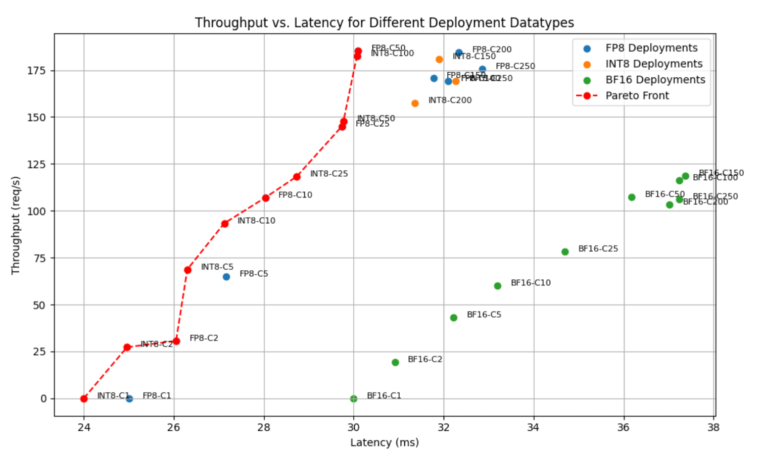
For a unit-cost model, record a candidate’s sustainable throughput under the relevant latency objective, not its highest observed throughput at any latency. Later lessons will examine saturation and tail latency in detail. For now, treat a benchmark as evidence supporting a capacity assumption, with its request mix and latency condition attached.

---

Build the inference-service model

Suppose a small online model runs on two replicas continuously for a 720-hour month. Each replica uses one accelerator and has benchmarked capacity of 10 requests per second at the required latency, with the expected request mix. Forecast demand averages 5.56 successful requests per second and peaks at 8. At that peak, one healthy replica could carry the load if the other failed; the second replica is not merely spare capacity to remove from the cost model.

Assume 14.4 million successful requests in the month, negligible billable failed attempts, and these illustrative, nonbundled rates:

Monthly component	Calculation	Cost
Two continuously provisioned replicas	2 × 720 hours × ($2 accelerator + $0.50 host) per hour	$3,600
Model storage and loading allocation	Fixed monthly estimate	$120
Shared serving-control services	Fixed monthly allocation	$120
Network and telemetry varying with requests	14.4 million × $0.00001 per request	$144
Total monthly serving cost		$3,984

Thus:

$$\text{Cost per successful request}=\frac{\$3,984}{14,400,000}\approx \$0.000277,$$

or about $0.277 per 1,000 successful requests. The fixed-plus-variable form is more useful than that single result:

$$C_{\text{month}}=nH(p_{\text{accelerator}}+p_{\text{host}})+C_{\text{model}}+C_{\text{shared}}+Q{c}_{\text{variable}}.$$

Here $n$ is provisioned replicas, $H$ is billed hours per replica, and $Q$ is successful requests under the example’s negligible-failure assumption. In a real ledger, charge attempt-based fees against attempts and divide the completed total by successes.

The average demand uses only about 28% of the fleet’s benchmarked request-handling capacity. That figure is not GPU utilization: it compares average request rate with the two-replica capacity of 20 requests per second. Some headroom pays for peaks and continued service after a replica failure. Removing it to improve average cost per request could violate the availability or latency requirement established earlier in this module.

If demand doubles, you cannot simply halve unit cost. First test whether the new peak still fits the fleet while meeting latency and failure-tolerance objectives. If it requires a third replica, the cost function jumps; it is not a smooth per-request discount. The same principle applies to training when a different accelerator count changes runtime, storage traffic, or scheduling wait.

---

Compare billing models without losing the workload

To make the price distinction concrete, imagine a comparable managed inference option. Assume each request uses 200 input tokens and 50 output tokens, with hypothetical prices of $0.60 per million input tokens and $2.40 per million output tokens. Its model-usage cost per request is:

$$c_{\text{managed}}=\frac{200(\$0.60)+50(\$2.40)}{1,000,000}=\$0.00024.$$

At 14.4 million requests, that is $3,456. If comparable application-side gateway, logging, and integration costs add a fixed $300 per month, the modeled total is $3,756, versus $3,984 for the self-hosted example. Do not add self-hosted accelerator costs to the managed price: the provider’s compute is already reflected in its usage charge.

Under the deliberately narrow assumption that request mix, unit rates, replica count, and peak requirement stay unchanged, you can express the two forecasts as:

$$C_{\text{self-hosted}}=\$3,840+\$0.00001Q,C_{\text{managed}}=\$300+\$0.00024Q.$$

They are equal at approximately 15.39 million requests per month. This is a scenario-specific crossover, not a purchasing rule. A changed prompt mix alters token cost; a higher peak may add a self-hosted replica; minimum commitments, discounts, transfer charges, quality, data requirements, and availability terms can change the comparison. A production decision requires comparable quality and service objectives on both sides.

For your operational cost ledger, the minimum useful measurements are billed replica- or accelerator-hours, actual job-attempt hours, successful and attempted request counts, request-size distribution, benchmarked throughput at the latency objective, chargeable transfer, artifact retention, and the rule for shared-cost allocation. Keep forecast, measured usage, and billed cost as separate fields. When they disagree, the difference tells you whether the workload assumption, performance benchmark, allocation, or price needs revision.

---

Conclusion

A unit-cost model is a defined accounting boundary applied to measured work—not simply a provider price divided by an estimate of traffic. For training, charge the resources and expected retry work needed to deliver an acceptable run. For inference, divide the complete period cost by successful requests while retaining the fixed capacity required for peaks, latency, and resilience. In both cases, document shared-cost allocations and report what the model excludes.

This completes the module’s path from workload requirements through architecture, capacity, and economics. Next, the course moves to reproducible workload foundations: packaging and versioning the code, data, and dependencies whose behavior these forecasts assume.