Tracing Data, Artifact, and Control Flows in End-to-End AI Systems

Hello! Last lesson turned an AI product requirement into measurable objectives for availability, latency, throughput, freshness, and quality. This lesson follows the system that must deliver those objectives. You’ll trace data as it is prepared and used, artifacts as they are built and released, and control decisions as they start, stop, or redirect work.

We’ll use the same recommendation service, with an optional generated explanation. The aim is not to memorize a particular platform diagram. It is to be able to look at any end-to-end AI architecture and answer: What moved across this boundary, what caused it to move, and which version was used?

---

Three flows occupy the same architecture

A conventional service diagram might show a request entering an API and a response leaving it. An AI system needs a wider view because the response depends on work done long before the request arrived.

Data flow carries information used or produced by the workload: activity events, labels, prepared features, prediction requests, retrieved documents, responses, and operational measurements. Some data is processed in bulk for training; other data must be available quickly for an online request.

Artifact flow carries durable, identifiable outputs that another step can reuse or release: a versioned dataset snapshot, a pipeline component image, a trained model package, an evaluation report, or a search index. A prepared dataset can be data from the trainer’s perspective and a versioned artifact from the pipeline’s perspective. The useful distinction is its role at a boundary, not its file extension.

Control flow determines whether, when, and with what configuration work happens. A schedule starts a training run; a validation result stops it; an approval makes a model eligible for deployment; a deployment specification tells serving replicas which model to load. A metric is observed data until a rule or person uses it to make a decision.

Watch the following overview with that distinction in mind. Although it demonstrates a particular pipeline framework, the important ideas are transferable: components consume inputs, produce artifacts, and record relationships between runs and outputs.

One infrastructure detail is worth making explicit. Metadata is not necessarily the artifact itself. A metadata store can record that training run run-318 produced a model at a particular object-storage location, along with the dataset and code versions it consumed. The large model files remain in artifact storage. Keeping that distinction clear makes lineage useful without turning the metadata service into a transfer path for every training byte.

---

Trace the candidate model from source data to release

The MLOps lifecycle image gives us a map of experimentation, automated pipelines, registry, serving, and monitoring. Its connecting lines combine several kinds of flow; we will separate them as we follow one candidate model.

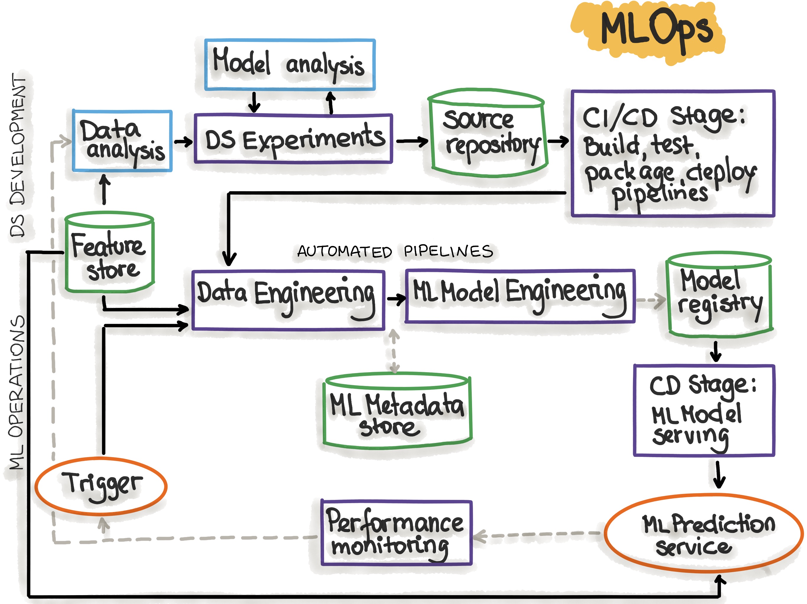
Suppose recent browsing activity helps rank recommended items. A particular training run might proceed as follows:

1. Collect and prepare data. Source systems supply activity events and, when available, later outcomes used as labels. Preparation checks schemas, applies transformations, and writes an identified training snapshot. The snapshot records a cutoff: activity arriving after that cutoff belongs to a later candidate, not silently to this one.
2. Build a candidate. A training job consumes that snapshot, a specified transformation implementation, training code, and configuration. It writes model files and a run record. The run record links to its inputs rather than merely saying “trained on recent data.”
3. Evaluate and decide. An evaluation job consumes the candidate model and an identified evaluation set. Its report contains quality results; the report is an artifact. A comparison against an acceptance rule is a control decision. If the rule fails, the candidate may remain available for investigation, but it does not become the serving model.
4. Register and release. A registry entry identifies the candidate model and its lineage. A separate release action selects an eligible model for a serving environment. Serving replicas obtain the specified model package and load it alongside compatible serving code.

Notice that training a model does not itself update a running prediction service. The candidate must pass a decision boundary, and the serving environment must be told what to load. Conversely, changing serving code does not automatically produce a newly trained model.

The reading below distinguishes delivery of a pipeline implementation from execution of that pipeline and delivery of its resulting model. Read its six stages as a list of outputs and decisions, rather than as a prescription for a particular cloud stack.

There is a useful DevOps distinction here. CI can build and test a new pipeline component image; delivery can install that component as part of a runnable pipeline. A later scheduled run can produce a different model version without another code change. These are separate release histories, so an incident record should say both which pipeline implementation produced a model and which model the serving service loaded.

---

Follow the live request without losing the training lineage

The request-time path is shorter than the model-development path, but it meets it at several points. An eligible recommendation request reaches the ingress measured in the previous lesson. The serving application obtains current features—for example, a recent-activity aggregate—from an online-accessible store. It applies the expected preprocessing, invokes the loaded model, and returns ranked items. A response record identifies the model version and, where practical, the feature version or snapshot it used.

Training and serving may read different representations of the same feature definition. Training needs historical values associated with the right examples and times; online serving needs low-latency access to current values. They should agree on meaning and transformation, but the model trained last week does not require every live request to use last week’s feature values. This is why “model version” alone cannot explain a recommendation.

The following compact trace shows what an operator would want to connect. The identifiers are illustrative; the point is the relationships, not a required logging format.

training run:     run-318
  data snapshot:  activity-snapshot-42
  transform:      features-6
  trainer image:  image-digest-91
  output model:   model-17
  evaluation:     eval-318 (passed release threshold)

serving release:  release-24
  model:          model-17
  server image:   image-digest-105

request:          req-9008
  release:        release-24
  feature read:   activity-feature-v6, updated_at=10:03:12
  outcome:        usable response
  ingress time:   184 ms

This record answers two different questions. “Why did this model behave this way?” leads through model-17 to its training inputs and evaluation. “Why was this request stale or slow?” leads through req-9008 to the feature read and serving release. A detailed production design would also account for sensitive data in request logs; linking versions does not require recording every raw user input.

The previous lesson’s objectives now have natural observation points. Availability and latency need request outcomes at ingress, not just successful model executions. Throughput needs offered traffic as well as completed work. Freshness needs the event’s creation time and the time its resulting feature became queryable. Quality needs evaluation and production feedback; an HTTP success cannot stand in for either.

---

Control decisions create the feedback loop

An end-to-end system is more than a one-time model-building sequence. Data availability, schedules, code changes, or observed degradation can initiate new work. But a trigger should not be confused with proof that new work is safe to release.

For example, a scheduled retraining run may start after new labels arrive. Before training, data validation can stop the run if required columns are missing. After training, model validation can stop promotion if quality falls below an accepted baseline or the package is incompatible with serving. The existing serving release can continue handling requests while the candidate is investigated. Monitoring might later propose another run, but that is another control event, not the monitoring data itself.

Read the sections below to see what must be recorded to reconstruct such decisions and what can trigger a new pipeline execution.

A practical trace therefore includes both what happened and what was permitted. If a new model is absent from production, investigate whether training failed, evaluation rejected it, registration did not complete, or release never selected it. Those are different failure domains even if the dashboard simply says “model not updated.”

---

Apply the same tracing method to a generative path

The optional generated explanation can use a retrieval-augmented generation (RAG) path. The image below shows document ingestion separately from processing a live query. Its details vary by implementation, but the separation is important.

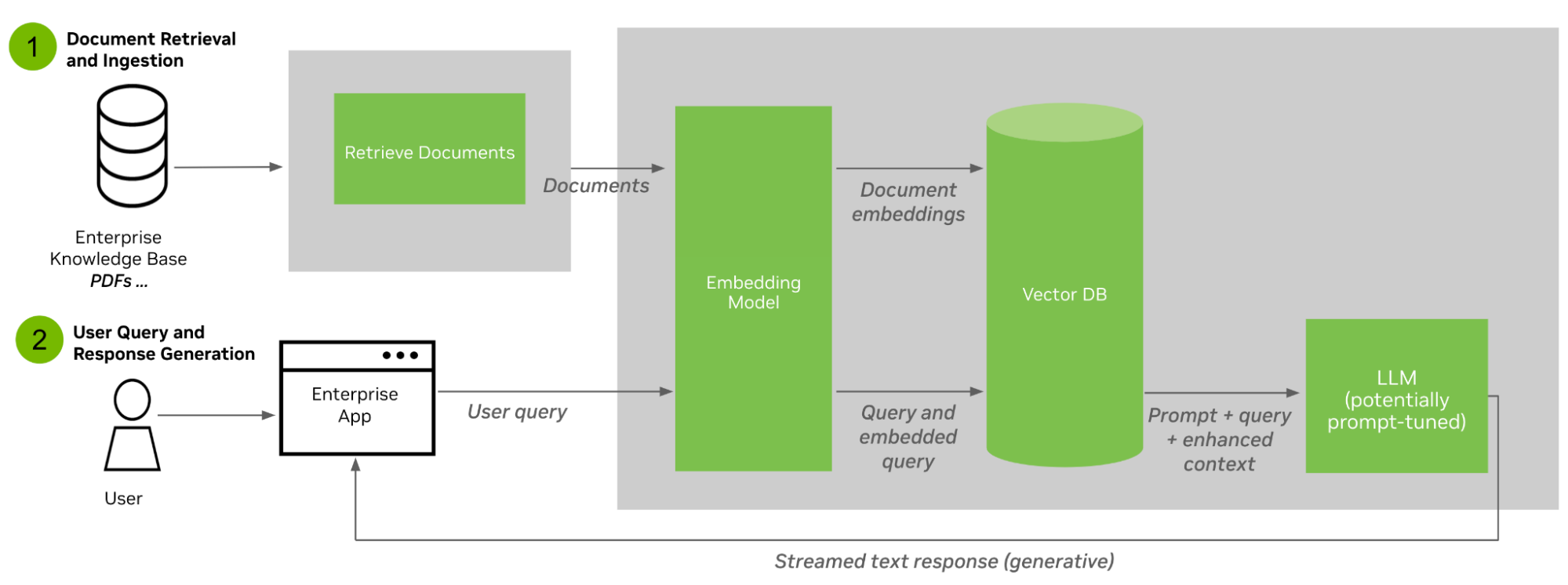
For ingestion, documents are retrieved from a source, processed, embedded, and made searchable. Here the searchable index is a materialized serving dataset and often a versioned artifact. Record which document collection, processing implementation, and embedding model produced it. Updating the index changes what answers can be grounded in, even if the generation model is unchanged.

For a live request, the application receives a question, obtains a compatible query embedding, retrieves relevant passages, assembles a prompt with those passages, and asks the LLM to generate an answer. The diagram compresses prompt assembly into its connections; in an implementation, the application or a retrieval service performs that work. The vector database supplies matches, not a finished prompt by itself.

The same three-flow test still works. Document text, retrieved passages, the query, and generated response are data. The embedding model, generation model, prompt template, and an identified index build can be artifacts. Rules that decide whether to refresh the index, which versions to deploy, and whether to accept a response are control. If an explanation cites obsolete item information, tracing only the LLM version will miss a potentially stale document index. If it is slow, request timing must distinguish retrieval from generation. This is the same diagnostic discipline used for recommendations, applied to a different request path.

---

Conclusion

An end-to-end AI system has interlocking histories. Data supplies training examples and live context; artifacts make prepared outputs, code, models, and indexes identifiable and reusable; control starts pipelines, enforces gates, and selects releases. A reliable trace joins those histories to the request the user experienced without assuming that a healthy service means fresh data or a good model.

Next, you’ll use this architectural trace to estimate compute, accelerator memory, network, and storage demands. Knowing which work happens where is the prerequisite for estimating how much infrastructure each path needs.