Characteristic Polynomials and Eigenvalues

Hello! Welcome back to our journey into eigenanalysis.

Introduction

In our last lesson, we established the fundamental concept of eigenvalues and eigenvectors, understanding them as the invariant directions and corresponding scaling factors of a linear transformation. We concluded with a crucial algebraic insight: a scalar $\lambda$ can only be an eigenvalue of a matrix $A$ if the matrix $(A-\lambda I)$ is singular. This led us to the all-important characteristic equation:
$\det (A-\lambda I)=0$
This equation bridges the gap between the geometric idea of an eigenvector and a concrete computational method for finding eigenvalues.

Today, we will focus entirely on this equation. Our goal is to derive the characteristic polynomial of a matrix and use it to compute eigenvalues. We will formalize the expression $\det (A-\lambda I)$, see that it is indeed a polynomial in $\lambda$, and develop a systematic procedure for finding its roots, which are the eigenvalues of our matrix.

1. The Characteristic Polynomial

The expression $\det (A-\lambda I)$ is a function of the variable $\lambda$. For an $n\times n$ matrix $A$, this function is a polynomial of degree $n$. This is called the characteristic polynomial of $A$. The eigenvalues are, by definition, the roots of this polynomial.

Properties of the Characteristic Polynomial

For an $n\times n$ matrix $A$, the characteristic polynomial, denoted $p_A(\lambda )=\det (A-\lambda I)$, has several important properties that can serve as a useful check on your calculations.

To summarize the key points for an $n\times n$ matrix $A$:

• The characteristic polynomial $p_A(\lambda )$ is a polynomial of degree $n$.
• The term with the highest power of $\lambda$ is $(-1{)}^n{\lambda }^n$.
• The coefficient of the ${\lambda }^{n-1}$ term is $(-1{)}^{n-1}\text{tr}(A)$, where $\text{tr}(A)$ is the trace of $A$ (the sum of its diagonal elements).
• The constant term (the ${\lambda }^0$ term) is $p_A(0)=\det (A-0I)=\det (A)$.

2. The 2x2 Case: A Practical Shortcut

For a 2x2 matrix, these properties give us a direct and fast way to find the characteristic polynomial. Let $A=\left(\begin{array}{cc}a& b\\ c& d\end{array}\right)$.

The polynomial is of degree 2, and we can write it as:
$p_A(\lambda )={\lambda }^2-(a+d)\lambda +(ad-bc)$
Or, more elegantly:
$p_A(\lambda )={\lambda }^2-\text{tr}(A)\lambda +\det (A)$
Setting this to zero gives the characteristic equation for any 2x2 matrix.

3. The General Case: $n\times n$ Matrices

For matrices larger than 2x2, we can't use the simple trace-determinant formula. We must compute the determinant $\det (A-\lambda I)$ directly, typically using cofactor expansion. This results in a polynomial of degree $n$, which can be challenging to solve.

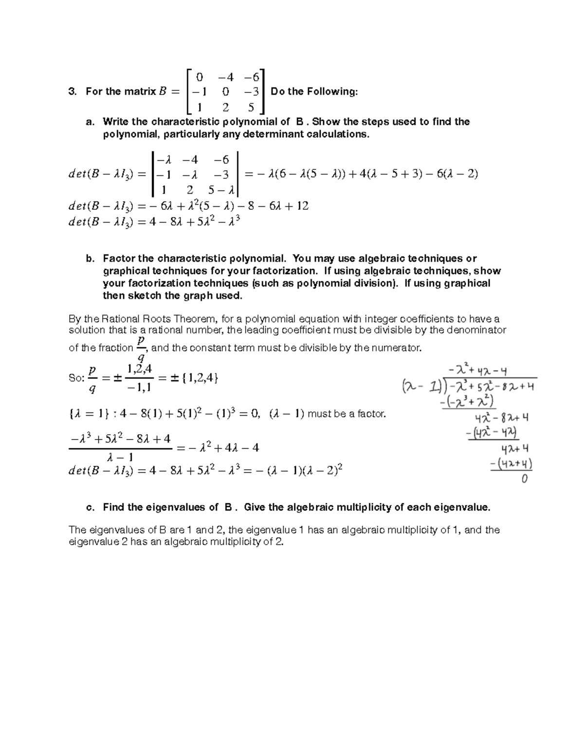
After finding the polynomial, the next step is to find its roots. For polynomials of degree 3 or higher, this often requires specific techniques. If the matrix has integer entries, the Rational Root Theorem is very useful. It states that any rational root of a polynomial with integer coefficients must be a divisor of the constant term.

This image provides a complete, handwritten walkthrough for a 3x3 matrix, demonstrating the full process from cofactor expansion to finding the roots.

4. A Special Case: Triangular Matrices

There is an important case where eigenvalue calculation becomes trivial. If a matrix is upper- or lower-triangular, its eigenvalues are simply the entries on its main diagonal.

For example, for the matrix:

The characteristic polynomial is $(3-\lambda )(-1-\lambda )(3-\lambda )=0$. The eigenvalues are immediately seen to be ${\lambda }_1=-1$ and ${\lambda }_2=3$ (with an algebraic multiplicity of 2, a concept we will explore later).

Conclusion

In this lesson, we have built the complete computational procedure for finding the eigenvalues of a square matrix. You learned to move from the abstract condition $\det (A-\lambda I)=0$ to a concrete polynomial whose roots give us the values we seek.

Key Takeaways:

• The characteristic polynomial of an $n\times n$ matrix $A$ is $p_A(\lambda )=\det (A-\lambda I)$, a polynomial of degree $n$.
• The roots of the characteristic polynomial are the eigenvalues of $A$.
• For a 2x2 matrix, the characteristic equation has a convenient form: ${\lambda }^2-\text{tr}(A)\lambda +\det (A)=0$.
• For larger matrices, we typically use cofactor expansion to find the polynomial and techniques like the Rational Root Theorem to find its roots.
• For any triangular matrix, the eigenvalues are simply the entries on its main diagonal.

Preview of the Next Lesson:
Finding the eigenvalues is only half the battle. For each eigenvalue $\lambda$ we've found, there is a corresponding set of eigenvectors. In the next lesson, we will complete the process by taking our computed eigenvalues and plugging them back into the equation $(A-\lambda I)\mathbf{x}=0$ to find the eigenvectors $\mathbf{x}$ that form the null space of that matrix.