Identifying Liquidity Traps: An IS-LM Approach

Hello! Welcome to the fifth and final lesson of our first module on deflation.

Introduction

In our previous lesson, we explored the Fisher Equation and conducted an empirical analysis showing how, during the Great Depression, deep deflation caused ex-post real interest rates to spike to punishingly high levels, even as the Federal Reserve cut nominal rates to near zero. This perverse dynamic, where monetary policy loses its ability to control the real cost of borrowing, sets the stage perfectly for today's topic.

This lesson addresses the final learning outcome of our introductory module: "Formulate empirical criteria for identifying a liquidity trap based on the IS-LM framework, focusing on the zero lower bound and interest elasticity of money demand."

We will define the liquidity trap, visualize it using the IS-LM model you're familiar with from your economics studies, and then evolve the concept to its modern interpretation. Most importantly, we will synthesize this theory into a practical, empirical toolkit for identifying when an economy might be caught in such a trap.

This lesson should take approximately 60 minutes to complete.

Recap from Last Lesson:

• We established that at the Zero Lower Bound (ZLB), the real interest rate $r$ is dictated by the rate of deflation ($\pi$), as $r\approx -\pi$.
• This means deeper deflation leads to higher real interest rates, a dynamic that chokes investment and exacerbates a downturn. This is the situation where conventional monetary policy becomes powerless.

1. The IS-LM Framework and the "Classic" Liquidity Trap

The concept of a liquidity trap was famously formalized by John Hicks in his 1937 IS-LM model as a way to interpret J.M. Keynes's arguments about the potential for an economy to get stuck in a persistent slump.

To build our understanding on a modern foundation, let's first review an updated IS-LM model. The following paper from the Dallas Fed provides a crisp derivation.

An IS-LM Analysis of the Zero-Bound Problem (The IS Curve; The LM Curve)
Reading time: ~10 minutes. Please read the sections on "The IS Curve" and "The LM Curve".

As you read, focus on these key points:

• The IS Curve: Note its derivation from intertemporal consumption choices and its dependence on the real interest rate (which incorporates inflation expectations).
• The LM Curve: Pay close attention to its construction. The crucial feature for our purposes is the kink, which creates a horizontal segment at the prevailing floor for interest rates (in this model, the interest paid on reserves, $I{R}_t$, which is effectively zero in many historical cases).

This horizontal section of the LM curve is the graphical representation of the liquidity trap.

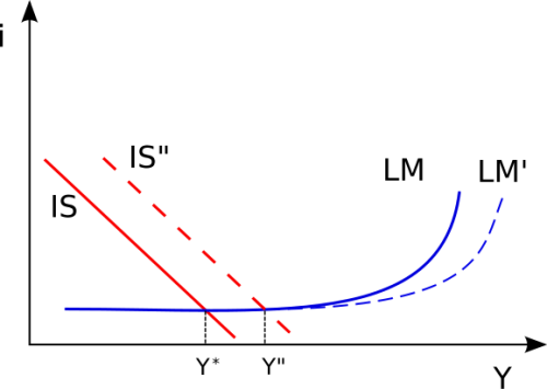This IS-LM diagram shows the LM curve becoming horizontal at a low interest rate. At this point, the demand for money is perfectly elastic, and increases in the money supply (shifting LM to the right) fail to lower the interest rate further.

What does this flat section mean?
It signifies that the interest elasticity of money demand has become infinite. At such low nominal interest rates, the opportunity cost of holding cash is virtually zero. Economic agents become indifferent between holding money (cash) and holding interest-bearing assets (bonds), as both offer a near-zero return. Consequently, any new money injected into the economy by the central bank is simply hoarded rather than used to buy bonds. This hoarding prevents bond prices from rising and, therefore, interest rates from falling.

The policy implication is stark. Please read the next short section of the same paper, which illustrates the trap.

An IS-LM Analysis of the Zero-Bound Problem (Equilibrium and the Zero Bound)
Reading time: ~3 minutes. Focus on Figure 7B and 7C and the accompanying text. This demonstrates why conventional monetary policy—shifting the LM curve by increasing the money supply—becomes ineffective.

When the IS curve intersects the LM curve on this horizontal segment, the economy is in a liquidity trap. The central bank can expand the monetary base (shifting LM to the right), but it will not lower the interest rate or stimulate aggregate demand. Monetary policy is like "pushing on a string."

2. The Modern View: It's All About Expectations

The classic IS-LM model is a powerful illustration, but modern macroeconomics, particularly the work of Paul Krugman in the late 1990s analyzing Japan, has refined the concept. The focus shifts from the mechanics of money demand to the role of expectations and the natural rate of interest.

Given your background, you'll appreciate the intellectual history and theoretical rigor in the following academic paper. Please read the section on the modern approach.

The IS-LM Model and the Liquidity Trap Concept (The Recent Approach to the Liquidity Trap (Krugman and Optimizing Models))
Reading time: ~10 minutes. This is a denser text. Focus on the key shifts in the modern framework:

1. The IS curve is explicitly a function of the expected real interest rate ($r=i-{\pi }^e$).
2. At the ZLB ($i=0$), this means the real rate is determined by expected inflation: $r\approx -{\pi }^e$.
3. A trap occurs when the Wicksellian "natural rate of interest"—the real rate needed to equilibrate saving and investment at full employment—becomes negative.

Let's unpack this. Imagine an economy is so depressed (perhaps due to a collapsed asset bubble or demographic shifts) that it requires a real interest rate of -2% to stimulate enough investment to return to full employment.

However, the nominal rate $i$ cannot go below zero. If everyone expects zero inflation (${\pi }^e=0$), the lowest possible real rate is $r=0\%-0\%=0\%$. This is higher than the required -2%, so the economy remains stagnant.

Worse, if the slump leads to expectations of deflation, say ${\pi }^e=-1\%$, the minimum real rate becomes $r\approx 0\%-(-1\%)=+1\%$. The economy needs a -2% rate, but the ZLB combined with deflationary expectations forces a real rate of +1%. This is precisely the perverse dynamic we saw in the last lesson, now framed as a primary condition for a liquidity trap.

In this modern view, the trap isn't just about the interest elasticity of money demand. It's a more fundamental problem where the equilibrium real interest rate required by the economy is unattainable because of the ZLB.

3. Formulating Empirical Criteria for a Liquidity Trap

Your learning outcome requires you to formulate empirical criteria for identifying a trap. This means moving beyond the diagrams to a checklist of observable economic data. Based on the theory we've covered, here is a set of criteria.

The following short video provides a fantastic, concise list of observable signs.

Viewing time: ~1 minute. Pay close attention to the five signs of a liquidity trap mentioned starting at 03:40.

Synthesizing the video and our other resources, we can formulate a comprehensive set of empirical criteria:

1. Prerequisite Condition:

• Near-Zero Short-Term Nominal Interest Rates: The policy rate (e.g., the Fed Funds Rate) is at or near the ZLB. This is the defining entry point for a potential trap.

2. Monetary Policy Ineffectiveness:

• Decoupling of Monetary Base and Broader Aggregates: Large-scale asset purchases (Quantitative Easing) lead to a massive increase in the monetary base, but this fails to translate into proportional growth in broader money supply (M2) or bank credit.
• Explosion in Excess Reserves: Commercial banks, instead of lending out the new liquidity, simply park it as excess reserves at the central bank. This was a prominent feature of the post-2008 landscape, as noted in the Jacob Clifford video.
  

3. Core Theoretical Indicators:

• Collapsing Velocity of Money: As people and firms hoard cash rather than spend or invest it, the velocity of circulation ($V$ in $MV=PY$) plummets. As you saw two lessons ago, this happened dramatically during the Great Depression.
• Persistently Low or Negative Inflation Expectations: Despite massive monetary easing, inflation remains stubbornly low, and measures of expected inflation (from surveys or inflation-indexed bonds like TIPS) are anchored at very low levels or indicate deflation. This is a sign that the central bank has lost credibility in its ability to generate inflation.

4. Real Economy Outcomes:

• Persistent Negative Output Gap: The economy operates significantly below its potential, with high unemployment and low capacity utilization, even with zero interest rates. This suggests the "natural" rate of interest is negative and unattainable.
• Stagnant Private Investment and Lending: Despite the low cost of borrowing, businesses are unwilling to invest, and banks are unwilling to lend, due to poor expectations about future growth and profitability.
• Deferred Consumption: While harder to measure directly, a general reluctance of households to spend on durable goods can be an indicator.

An economy exhibiting most or all of these symptoms simultaneously is very likely in a liquidity trap.

Conclusion

Today, we have traced the liquidity trap from its classic formulation in the IS-LM model to its modern interpretation centered on expectations and the natural rate of interest. You are now equipped not just with the theory but with a concrete set of empirical criteria to diagnose this challenging macroeconomic state.

Key Takeaways:

• A liquidity trap is a state where conventional monetary policy becomes ineffective because nominal interest rates are at the Zero Lower Bound.
• Graphically, this is represented by the horizontal portion of the LM curve, where the interest elasticity of money demand is infinite.
• The modern view emphasizes that a trap occurs when the natural rate of interest is negative, and deflationary expectations keep the real interest rate stuck above it.
• Empirical criteria for identifying a trap include: near-zero policy rates, ineffective monetary easing (evidenced by soaring excess reserves), collapsing money velocity, persistent low inflation expectations, and a stagnant real economy (high unemployment, low investment).

Preview of the Next Module:

This lesson concludes our first module on the essential empirical frameworks for analyzing deflation. You now have a toolkit comprising the Quantity Theory of Money, the Fisher Equation, and the IS-LM model of a liquidity trap.

In our next module, "The Deflation Debate and Historical Precedent," we will begin to apply these tools. We will start by tackling a crucial question: Is all deflation bad? We will analyze the distinction between 'good' (supply-side) and 'bad' (demand-side) deflation, setting the stage for our deep dive into the Great Depression.