Recommended resources
The freely available resources this lesson will direct you to.
Hello! Welcome back to our module on giving agents a knowledge base.
In our previous lesson, we established the "why" and "what" of Retrieval-Augmented Generation (RAG). We saw that RAG is an architectural pattern that turns a "closed-book" LLM into an "open-book" reasoner, solving critical issues like knowledge cutoff and hallucination by grounding the model's responses in external, verifiable information.
Today, we dive into the heart of the "retrieve" step. The performance of your entire RAG system hinges on its ability to find the most relevant information for a given query. This retrieval process depends on two core components: embedding models and distance metrics. Our goal in this lesson is to analyze the impact of different embedding models and distance metrics on retrieval performance and cost.
Making the right choices here is a fundamental architectural decision. For your goal of delivering agentic AI solutions to clients, understanding these trade-offs will allow you to design systems that are not only accurate but also cost-effective and scalable.
1. From Text to Vectors: The Role of Embedding Models
The first step in making knowledge searchable is to convert it into a format that a machine can understand and compare. We do this by transforming text into numerical vectors, or embeddings. An embedding is a point in a high-dimensional space where the distance between points represents semantic similarity.
An embedding model is a specialized neural network, typically a Transformer, that has been trained to perform this transformation. It reads text and outputs a dense vector. To understand how the design of these models impacts performance, we first need to look at their architecture.
Embedding Models: Architecture, Pooling & Selection
This article provides an excellent, interactive breakdown of embedding model architecture. It will give you the foundational knowledge needed to understand the design choices behind different models.
Please read the introduction and the first two main sections, 'Embedding Model Architectures' and 'Pooling Strategies'. Focus on: The concept of a 'bi-encoder' and why it's efficient for retrieval. The critical role of the 'pooling layer' in converting token-level information into a single sentence-level vector. Pay close attention to the differences between CLS Pooling and Mean Pooling.
As you've just read, a key step is pooling, which aggregates the sequence of token-level vectors produced by the Transformer into a single vector for the entire text chunk. The choice of pooling strategy (e.g., averaging all token vectors vs. using a special [CLS] token) is not arbitrary; it's tied to how the model was trained. Using the wrong pooling strategy for a given model will degrade retrieval quality.
To see this in action, the article you just read contains a practical code demonstration.
Embedding Models: Architecture, Pooling & Selection
This interactive section of the same article demonstrates how different pooling strategies affect similarity scores for a model trained with a specific strategy.
Now, review the code and the resulting heatmaps in the 'Comparing Pooling Strategies' part of the article (located after the descriptions of the individual pooling strategies). You don't need to run the code yourself, but observe how the 'mean_sims' heatmap correctly identifies the two similar sentences, while the other strategies fail to do so as effectively for this particular model.
This illustrates a crucial point for system design: an embedding model is not just a black box. Its internal architecture and training process dictate how it should be used.
2. The Performance-Cost Trade-off in Embedding Models
Now that we understand the basic architecture, let's analyze the factors that influence the performance and cost of an embedding model. This is where you'll make key design decisions when building a system for a client.
Factor 1: Embedding Dimensionality
The length of the vector produced by the model—its dimensionality—is a primary factor in the performance-cost equation.
- Higher dimensions can capture more nuance, potentially leading to better retrieval quality.
- Lower dimensions result in smaller vector sizes, which reduces storage costs and can speed up similarity searches.
The article we've been using provides a clear overview of this trade-off.
Embedding Models: Architecture, Pooling & Selection
Let's continue with the same article to explore the impact of dimensionality.
Read the section 'Embedding Dimensions'. Pay attention to the table of common dimensionalities and the explicit breakdown of the trade-offs (Storage, Computation, Indexing).
A sophisticated technique called Matryoshka Representation Learning (MRL) allows a single model to offer flexible dimensionality, giving you more control over this trade-off without needing multiple models.

This is a powerful feature for production systems. You could use a shorter, faster version of the embedding for an initial, broad search, and then re-rank the top results using the full-dimensional, more accurate embedding. Let's see MRL in action.
Embedding Models: Architecture, Pooling & Selection
The article demonstrates MRL with a practical example, showing how retrieval quality improves as dimensionality increases.
Study the code example and the bar chart visualization under the 'Matryoshka Representation Learning' subsection. Notice how the model correctly identifies the most relevant document even at 64 dimensions, but the separation between relevant and irrelevant documents becomes much clearer at higher dimensions.
Factor 2: Model Size and Selection Tiers
Larger models with more parameters generally produce higher-quality embeddings but are slower and more expensive to run. The choice of model often falls into one of three practical tiers.
Embedding Models: Architecture, Pooling & Selection
The final sections of the article provide a framework for model selection.
Read the sections 'Embedding Model Selection', 'Evaluating on Your Own Data', and 'API-Based Embedding Models'. Focus on the 'Practical Model Tiers' (Lightweight, Mid-range, Heavy) and the importance of evaluating models on your own domain-specific data, not just relying on general benchmarks like MTEB.
Factor 3: Compression and Quantization
Beyond choosing a model and dimensionality, we can further optimize for cost by compressing the embedding vectors. While embedding computation is relatively cheap, storing billions of high-dimensional vectors can lead to substantial operational costs.
The Hidden Cost of Embeddings in RAG and how to Fix it
This video provides a clear, high-level explanation of why embedding storage is a 'hidden cost' and introduces the two main strategies to combat it: dimensionality reduction and quantization.
Watch from the beginning to 09:38. The video explains the storage cost calculation and then introduces quantization (reducing precision, e.g., from 32-bit to 8-bit floats) as a powerful compression technique. Pay attention to the study results showing that quantization can dramatically reduce storage with minimal impact on retrieval accuracy.
The video introduces key concepts. For a deeper, more rigorous analysis suitable for your background, we'll turn to a recent research paper that systematically investigates these optimization techniques.
[PDF] Optimization of embeddings storage for RAG systems using...
This research paper offers a systematic comparison of compression techniques, providing the kind of empirical evidence needed for making robust architectural decisions.
Please review the following sections of the paper: Abstract (Section 0): Get a high-level summary of the findings. Section 5.1, 'Impact of Quantization' (Section 3): Note the comparison between float16, int8, and the novel float8 formats. The key insight is that float8 provides a 4x reduction with negligible performance loss, outperforming the more common int8. Section 5.2, 'Impact of Dimensionality Reduction Methods' (Section 4): This section confirms that PCA is the most effective and practical method. Section 5.3, 'Combined Effects of Quantization and PCA' (Section 5): This is the crucial synthesis. Focus on the conclusion that combining moderate PCA with float8 quantization offers an excellent trade-off, achieving high compression with minimal performance loss. Review Table 1 to see the concrete numbers. Section 6, 'Conclusions' (Section 7): Read the bullet points for a concise summary of the paper's takeaways.
The key takeaway from this research is that you have a powerful toolkit for managing the cost-performance trade-off. For a client project, you could start with a high-quality model and then apply techniques like float8 quantization and PCA to meet specific budget or hardware constraints, armed with data to show the minimal impact on performance.
Modern embedding models often integrate several of these advanced features.
The Only Embedding Model You Need for RAG
To see how these concepts come together in a state-of-the-art model, let's look at a video discussing the Jina V4 embedding model.
Watch from 01:33 to 03:08 and from 04:25 to 07:26. Notice how this single model architecture incorporates many of the ideas we've discussed: Support for both dense (single-vector) and multi-vector representations. Task-specific embeddings via LoRAs. Matryoshka embeddings for variable output dimensions, which directly impacts cost and speed.
3. Measuring Similarity: The Role of Distance Metrics
Once we have our document corpus represented as a collection of embedding vectors, retrieval becomes a nearest-neighbor search problem. Given a query vector, we want to find the document vectors that are "closest" in the embedding space. This "closeness" is measured by a distance metric.
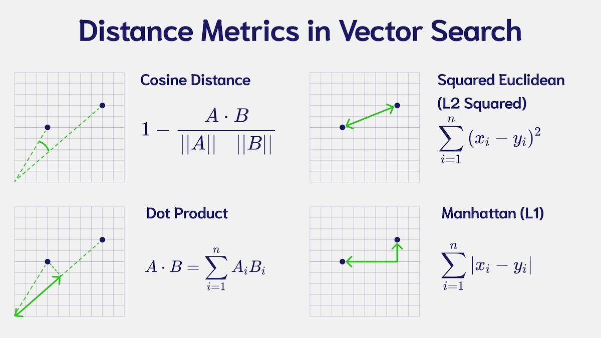
- Cosine Similarity: Measures the cosine of the angle between two vectors. It ranges from -1 (opposite) to 1 (identical). It's effective because it only considers the orientation of the vectors, not their magnitude.
- Euclidean Distance (L2): The straight-line "ruler" distance between the two vector endpoints.
- Dot Product: A measure of one vector's projection onto another.
The choice of metric is not arbitrary; it's linked to the model's training. Most modern embedding models are optimized for cosine similarity. There's a crucial implementation detail that simplifies this calculation: normalization.
Embedding Models: Architecture, Pooling & Selection
This final section from our main article explains why normalization is a standard and important post-processing step.
Read the short section 'Normalization and Post-Processing'. The key insight is that by normalizing all vectors to unit length (L2 norm = 1), the computationally expensive cosine similarity calculation becomes equivalent to a simple dot product. This is a standard optimization in all vector databases.
For practical purposes, this means that for most RAG systems you build, you will:
- Generate embeddings using a model designed for cosine similarity.
- L2-normalize all vectors before storing them.
- Use the dot product as your similarity function during retrieval, as it will be mathematically equivalent to cosine similarity and computationally faster.
Conclusion
In this lesson, we dissected the core components of the retrieval step in RAG. You now have a framework for analyzing the critical architectural decisions that balance retrieval performance against system cost.
Here are the key takeaways:
- Model Architecture Matters: An embedding model's design (e.g., pooling strategy) dictates how it should be used.
- A Multi-Factor Trade-off: Selecting an embedding model involves balancing performance (driven by model size and architecture) with cost (driven by dimensionality, storage, and computation).
- Optimization is Key: Techniques like Matryoshka embeddings give you flexible dimensionality. Quantization (especially to
float8) and dimensionality reduction (PCA) are powerful tools for drastically reducing storage costs with minimal performance impact. - Use the Right Metric: Most models are trained for cosine similarity. By normalizing your vectors, you can use the faster dot product for retrieval, a standard and crucial optimization.
In our next lesson, we will move one step up in the design process. Now that we know how to encode and retrieve information effectively, we'll address a more strategic question: "Determine what business knowledge to include in a RAG knowledge base and what to exclude." This involves analyzing business processes to decide what information is valuable, what is noise, and how to structure it for optimal retrieval.