Saving and Restoring Training Checkpoints

Welcome back. Last lesson, you separated training from validation: model.train() selects training behavior, while model.eval() and torch.no_grad() help you measure a model without updating it. Now consider what happens if training must stop after an epoch. The model’s current weights are worth keeping, but weights alone may not be enough to continue the same optimization process.

In this lesson, you’ll save a checkpoint containing both model and optimizer state, load it into fresh objects, and perform another training update. The small example is self-contained, so you can run it even if you no longer have the previous notebook open.

A checkpoint captures more than predictions

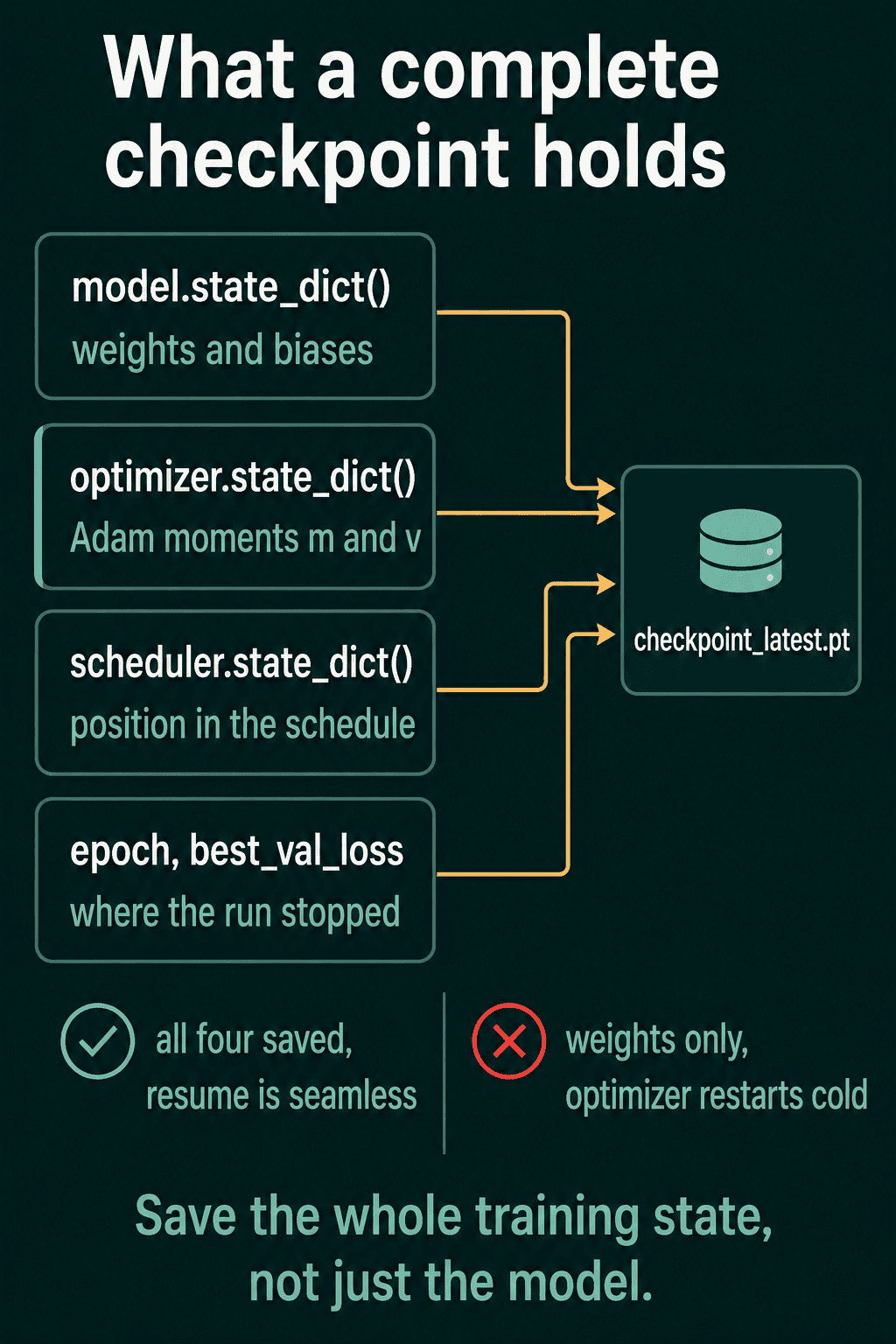
A model’s state_dict() contains its learned parameters and any registered buffers, such as batch-normalization running statistics. An optimizer has a separate state_dict() containing its settings and accumulated state. For Adam, that accumulated state includes estimates based on earlier gradients. If you restore only the model weights, you can make the same predictions immediately, but Adam starts again without that history.

A useful checkpoint also records where to resume, such as the next epoch number. If your training loop uses a learning-rate scheduler, its state belongs in the checkpoint too. The diagram shows these distinct pieces; our example will use a model, an optimizer, and epoch metadata, but no scheduler.

Watch the selected parts of Patrick Loeber’s PyTorch Tutorial 17 - Saving and Loading Models. Notice the difference between loading a model for predictions and loading a checkpoint for continued training.

The save-and-load contract

PyTorch’s Saving and Loading Models tutorial provides the reference pattern. Read its definition of a state dictionary and its general-checkpoint example. Pay particular attention to the order on loading: create a model and an optimizer, load their respective states, then select training or evaluation mode for what you will do next.

The checkpoint is an ordinary Python dictionary serialized with torch.save(). Its keys are names you choose; they need only match when you load them. We’ll store next_epoch rather than epoch so that the loop’s starting point is unambiguous: after completing epochs numbered 0 and 1, the next epoch is 2.

Save after a completed training epoch

The following MLP and training step use the same zero_grad(), backward(), and step() pattern you learned earlier. The tiny dataset exists only to make the checkpoint procedure runnable; two passes over it are not intended to produce a well-trained classifier.

import torch
from torch import nn

class MLP(nn.Module):
    def __init__(self):
        super().__init__()
        self.net = nn.Sequential(
            nn.Linear(4, 8),
            nn.ReLU(),
            nn.Linear(8, 3),
        )

    def forward(self, x):
        return self.net(x)

X = torch.tensor([
    [1., 0., 0., 0.],
    [0., 1., 0., 0.],
    [0., 0., 1., 0.],
    [2., 0., 0., 0.],
    [0., 2., 0., 0.],
    [0., 0., 2., 0.],
])
y = torch.tensor([0, 1, 2, 0, 1, 2], dtype=torch.long)

loss_fn = nn.CrossEntropyLoss()
model = MLP()
optimizer = torch.optim.Adam(model.parameters(), lr=1e-3)

def train_one_epoch(current_model, current_optimizer):
    current_model.train()
    current_optimizer.zero_grad()
    loss = loss_fn(current_model(X), y)
    loss.backward()
    current_optimizer.step()
    return loss.item()

for epoch in range(2):
    last_train_loss = train_one_epoch(model, optimizer)

checkpoint_path = "mlp_checkpoint.pt"
torch.save(
    {
        "next_epoch": epoch + 1,
        "model_state_dict": model.state_dict(),
        "optimizer_state_dict": optimizer.state_dict(),
        "last_train_loss": last_train_loss,
    },
    checkpoint_path,
)

print("Saved after epoch index", epoch)
print("Next epoch index:", epoch + 1)

Run the block through the save operation. The file is written after both the backward pass and optimizer step for epoch 1, so next_epoch correctly identifies the first epoch not yet run. Saving an epoch number without deciding whether it means “last completed” or “next to run” is an easy way to repeat or skip an epoch.

The loss is useful for a log, but restoring it does not restore training. The essential state for this example is the model, the Adam optimizer, and the loop position.

Restore into fresh objects, then continue

Run this second block after the first. It creates a new model with the same architecture and a new Adam optimizer attached to that model’s parameters. Loading the two state dictionaries then replaces their newly initialized state with the saved state.

resumed_model = MLP()
resumed_optimizer = torch.optim.Adam(
    resumed_model.parameters(), lr=1e-3
)

checkpoint = torch.load(
    checkpoint_path,
    map_location="cpu",
    weights_only=True,
)

resumed_model.load_state_dict(checkpoint["model_state_dict"])
resumed_optimizer.load_state_dict(
    checkpoint["optimizer_state_dict"]
)
start_epoch = checkpoint["next_epoch"]

# Check the restored state before performing another update.
assert all(
    torch.equal(saved, restored)
    for saved, restored in zip(
        model.parameters(), resumed_model.parameters()
    )
)

original_first_parameter = next(model.parameters())
restored_first_parameter = next(resumed_model.parameters())

assert torch.equal(
    optimizer.state[original_first_parameter]["exp_avg"],
    resumed_optimizer.state[restored_first_parameter]["exp_avg"],
)

print("Restored next epoch index:", start_epoch)
print("Restored learning rate:",
      resumed_optimizer.param_groups[0]["lr"])

# The saved loop position was 2, so this runs epoch index 2.
for epoch in range(start_epoch, 3):
    loss = train_one_epoch(resumed_model, resumed_optimizer)
    print(f"Completed epoch index {epoch}; loss = {loss:.4f}")

The first assertion compares model parameters. The second checks one of Adam’s saved moving-gradient estimates, demonstrating something a weights-only file could not restore. The resumed training function calls train() and performs a new gradient-tracked forward pass, just as it should after last lesson’s validation phase. It uses the restored optimizer, which is attached to resumed_model’s parameters; an optimizer still attached to the old model would update the wrong object.

map_location="cpu" makes this example load onto the CPU even if a checkpoint was saved from another device. For GPU training, the model, input tensors, and restored optimizer state must be placed consistently on the intended device. The weights_only=True option supports this dictionary of tensors and simple metadata while restricting what torch.load() will deserialize; still, load checkpoint files only from sources you trust.

What “resume” does—and does not—guarantee

This checkpoint lets the example continue with the saved parameters, Adam history, and correct epoch number. It does not save the previous autograd graph or pending .grad values; the next training step builds a new graph and computes new gradients. Nor does state_dict() save whether you last called model.train() or model.eval(). Set the appropriate mode after loading.

For a more elaborate run, save any other state needed to pick up its procedure: for example, a scheduler’s state and the best validation score used to decide which model to retain. A checkpoint taken at an epoch boundary is simpler to resume than one taken halfway through a shuffled data pass. Even with model and optimizer state restored, random operations or a different data order can cause subsequent updates to differ from an uninterrupted run. The next lesson addresses how to control randomness for a reproducible small experiment.

Conclusion

For continued training, save both model.state_dict() and optimizer.state_dict(), along with an unambiguous loop position. To resume, recreate the same model architecture and an optimizer bound to its parameters, load both states, switch to training mode, and continue from the recorded epoch. A weights-only file is useful for predictions, but it is not a complete record of a training run.