Optimization with Equality Constraints

Recommended resources

The freely available resources this lesson will direct you to.

Hello! In our last module, we completed our study of unconstrained optimization by proving the linear convergence rate of gradient descent for smooth and strongly convex functions. We now have a robust theoretical understanding of how to find the minimum of a function when our variables are free to take any value.

However, many real-world problems are not so simple. We often need to find the best solution while adhering to certain limitations or rules. This brings us to the next major topic in our course.

Introduction

This lesson begins our journey into Module 5: Constrained Optimization and Duality. Our first goal is to master the learning outcome: Formulate an optimization problem with equality constraints.

We will transition from the open landscapes of unconstrained problems to the more structured world where our solutions must satisfy specific equations. We will formally define the components of a constrained optimization problem—the objective function, the decision variables, and the equality constraints—and learn how to write them in a standard mathematical form. We'll also build a strong geometric intuition for how constraints alter the nature of the optimization problem.

This foundational step is crucial. Before we can learn to solve these problems, we must first learn how to describe them precisely.

Part 1: The Formal Language of Constrained Optimization

In unconstrained optimization, our goal was to find $x \in R^{n}$ that minimizes $f (x)$ . In constrained optimization, we add a crucial new element: a set of rules that $x$ must obey. Today, we focus on rules expressed as equalities.

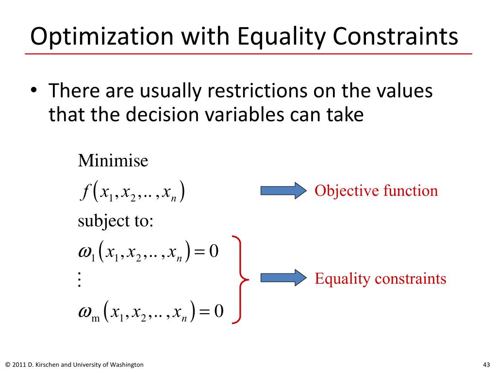
The standard formulation of an optimization problem with equality constraints is as follows:

Minimize: $f (x)$
Subject to:

g_{1} (x) g_{2} (x) g_{m} (x) = 0 = 0 ⋮ = 0

Let's break down the components:

Objective Function, $f (x)$ : This is the function $f : R^{n} \to R$ that we want to minimize (or maximize). It represents the cost, error, or quantity we are trying to optimize.
Decision Variables, $x$ : This is the vector $x = [x_{1}, x_{2}, \dots, x_{n}]^{T} \in R^{n}$ containing the variables we can control.
Equality Constraints, $g_{i} (x) = 0$ : These are $m$ functions, $g_{i} : R^{n} \to R$ , that define the conditions our solution must satisfy. We can compactly represent them as a single vector-valued function $g : R^{n} \to R^{m}$ , where $g (x) = 0$ .
Feasible Set: The set of all points $x$ that satisfy all constraints is called the feasible set, often denoted by $C$ . For our problem, $C = {x \in R^{n} ∣ g_{i} (x) = 0 for all i = 1, \dots, m}$ .

The optimization problem is then to find the point $x^{*}$ in the feasible set $C$ that has the smallest (or largest) value of $f$ .

Formulation of Optimization with Equality Constraints — This image shows the standard formulation of a constrained optimization problem. The function $f$ is our objective function, and the functions $g_i(\mathbf{x})$ (denoted here as $\omega_i$) are the equality constraints. Any constraint of the form $h(\mathbf{x}) = c$ can be rewritten in this standard form as $g(\mathbf{x}) = h(\mathbf{x}) - c = 0$.

To see these definitions presented in a formal context, please review the following text.

Constrained Optimization (Equality Constraints)

These lecture notes provide a clear and formal introduction to the framework of constrained optimization.

Please read Section 1, 'Preliminaries', and the first part of Section 2, titled 'Several Equality Constraints'. Focus on how the text defines the constraint set C and generalizes the problem from a single constraint g(x) = 0 to multiple constraints g_j(x) = 0, j=1,...,m.

Part 2: A Geometric Perspective

How does a constraint fundamentally change the problem?

In unconstrained optimization, we could search for the optimum across the entire domain $R^{n}$ . The optimum $x^{*}$ satisfied the condition $\nabla f (x^{*}) = 0$ .

With an equality constraint, we are no longer free to roam. We are restricted to a specific surface or curve defined by $g (x) = 0$ . This is the feasible set. It's highly likely that the unconstrained minimum of $f$ does not lie in this set.

Therefore, the constrained minimum will be a point on the feasible surface that achieves the lowest possible value of $f$ .

Multivariate Optimization with Equality Constraint — This diagram illustrates the core challenge. The concentric ellipses are the contour lines of an objective function $f(x_1, x_2) = x_1^2 + 4x_2^2$. The unconstrained minimum is at the center (0,0). The straight line represents a linear equality constraint, which is the feasible set. The solution to the constrained problem is not the unconstrained minimum; it must be a point that lies on the line.

This visualization highlights the trade-off: we want to get to the "bottom of the valley" (the center of the ellipses), but we are forced to stay on the "path" defined by the constraint line. The optimal point will be where the path gets closest to the bottom of the valley.

The following video provides an excellent animated introduction to this idea.

Lec 13: Constrained Optimization I: Equality constraints

This video from NPTEL provides a clear graphical explanation of how an equality constraint restricts the solution space.

Watch the segment from 04:18 to 06:23. The lecturer uses a contour plot to show how the minimum point shifts from the unconstrained optimum to a new point on the constraint line, which represents the feasible region.

Part 3: Formulating a Problem

Let's ground this with a concrete example that connects to your background in machine learning.

Imagine you are building a financial portfolio of two assets. Your goal is to minimize the portfolio's risk, while achieving a specific target expected return.

Let $x = [x_{1}, x_{2}]^{T}$ be the weights of the two assets in your portfolio.
The portfolio's risk (variance) is given by an objective function $f (x_{1}, x_{2}) = σ_{1}^{2} x_{1}^{2} + σ_{2}^{2} x_{2}^{2} + 2 ρ σ_{1} σ_{2} x_{1} x_{2}$ , where $σ_{i}$ are the asset volatilities and $ρ$ is their correlation. This is a quadratic function of $x$ .
Your first constraint is that the weights must sum to 1: $x_{1} + x_{2} = 1$ .
Your second constraint is that the portfolio's expected return must equal a target value, $R$ . The expected return is $μ_{1} x_{1} + μ_{2} x_{2}$ , where $μ_{i}$ are the individual asset returns. So, $μ_{1} x_{1} + μ_{2} x_{2} = R$ .

How do we formulate this as a standard optimization problem?

Objective Function:
$Minimize f (x_{1}, x_{2}) = σ_{1}^{2} x_{1}^{2} + σ_{2}^{2} x_{2}^{2} + 2 ρ σ_{1} σ_{2} x_{1} x_{2}$
Constraints: We rewrite the constraints in the standard $g (x) = 0$ form.
$g_{1} (x_{1}, x_{2}) = x_{1} + x_{2} - 1 = 0$
$g_{2} (x_{1}, x_{2}) = μ_{1} x_{1} + μ_{2} x_{2} - R = 0$

This complete formulation precisely describes the famous Markowitz mean-variance optimization problem, a cornerstone of modern portfolio theory.

Test your understanding!

You are tasked with designing a rectangular container with length $l$ , width $w$ , and height $h$ . Your goal is to maximize the volume of the container. However, due to material limitations, the total surface area of the container must be exactly $A_{0}$ .

Formulate this as a constrained optimization problem. Identify the objective function, the decision variables, and the equality constraint function.

Show answer

Decision Variables: The vector of variables we can control is $x = [l, w, h]^{T}$ .
Objective Function: We want to maximize the volume, $V = l w h$ . So, our objective function is $f (l, w, h) = l w h$ .
Equality Constraint: The surface area of a rectangular box is $2 (l w + l h + w h)$ . This must be equal to $A_{0}$ .
$2 (l w + l h + w h) = A_{0}$
To write this in standard form, we define the constraint function $g$ :
$g (l, w, h) = 2 (l w + l h + w h) - A_{0} = 0$
Full Formulation:
[
\begin{align*}
\text{Maximize } & f(l, w, h) = lwh \
\text{Subject to } & g(l, w, h) = 2(lw + lh + wh) - A_0 = 0
\end{align*}
\end{align*}
We would also have implicit constraints $l, w, h > 0$ , which are inequality constraints, a topic for a future lesson. For now, we focus on the equality constraint.

Conclusion

In this lesson, we have laid the formal groundwork for studying a new and important class of optimization problems.

Key Takeaways:

A constrained optimization problem consists of an objective function to minimize or maximize, subject to a set of constraints.
Equality constraints take the form $g_{i} (x) = 0$ . A problem can have multiple such constraints.
The feasible set is the collection of all points $x$ that satisfy all constraints. The solution to the problem must lie within this set.
Geometrically, constraints restrict the search space from the entire domain $R^{n}$ to a lower-dimensional surface or curve, meaning the unconstrained optimum is generally not a valid solution.

Preview of the Next Lesson:
Now that we can formally state a problem with equality constraints, the natural next question is: how do we solve it? In our next lesson, we will derive the celebrated method of Lagrange multipliers. This powerful technique provides a necessary condition for optimality in constrained problems by analyzing the relationship between the gradient of the objective function and the gradients of the constraint functions at an optimal point.