Optimizing with Inequality Constraints

Recommended resources

The freely available resources this lesson will direct you to.

Hello! Welcome back to our course.

In our previous lesson, we mastered the method of Lagrange multipliers to solve optimization problems with equality constraints. We saw that at a constrained optimum, the gradient of the objective function is parallel to the gradient of the constraint function. This insight allowed us to set up and solve a system of equations to find candidate solutions.

Today, we move to a more general and widely applicable class of problems. Our learning outcome is to formulate an optimization problem with inequality constraints. This is a critical step because most real-world problems in machine learning and engineering involve constraints like budgets, resource limits, or physical boundaries, which are best described by inequalities (e.g., "cost $\leq$ $100," "power $\geq$ 0").

We will explore why the simple parallelism of gradients is no longer sufficient and introduce the foundational concepts needed to handle these new complexities. This lesson will build the conceptual bridge from Lagrange multipliers to the powerful Karush-Kuhn-Tucker (KKT) conditions, which we will derive in our next session.

1. The Standard Formulation of a Constrained Problem

An optimization problem with inequality constraints has a different character from one with only equality constraints. Let's start by defining the standard form. A general (minimization) problem is written as:

General Optimization Problem Formulation — A standard representation of a constrained optimization problem. The goal is to minimize an objective function $f(\mathbf{x})$ while satisfying a set of equality constraints $h_i(\mathbf{x})=0$ and inequality constraints $g_j(\mathbf{x}) \le 0$.

The components are:

Objective function, $f (x)$ , which we want to minimize.
Inequality constraints, $g_{j} (x) \leq 0$ .
Equality constraints, $h_{k} (x) = 0$ .

A Note on Convention:
For consistency, we will adhere to this standard form.

A maximization problem maximize f(x) can be converted to minimization by minimizing $- f (x)$ .
An inequality like $g (x) \geq 0$ can be converted by multiplying by -1 to get $- g (x) \leq 0$ .

The set of all points $x$ that satisfy all constraints is called the feasible set, often denoted by $Ω$ . Unlike an equality constraint like $x^{2} + y^{2} = 1$ which confines you to a circle (a 1D curve in 2D space), an inequality constraint like $x^{2} + y^{2} \leq 1$ defines a whole region (a 2D disk).

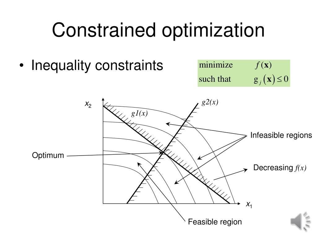
Constrained Optimization with Inequality Constraints — This image illustrates the feasible region for a minimization problem. The solution (optimum) must lie within this region, which is defined by the inequality constraints $g_1(\mathbf{x}) \le 0$ and $g_2(\mathbf{x}) \le 0$.

To formalize this, please read the following brief definitions.

EE5121 Optimization - Constrained Optimization

This resource from IIT Madras provides precise definitions for the 'feasible set' and the 'active set', which are fundamental terms in constrained optimization.

Please read the first two subsections, 'Feasible set' and 'Active set'. Focus on how the feasible set \Omega is defined and understand the definition of an 'active' constraint (c_i(\mathbf{x}) = 0).

2. The Crucial Idea: Active vs. Inactive Constraints

The core challenge of inequality constraints is that we don't know in advance whether the optimal solution will be in the interior of the feasible region or on its boundary. This leads to two distinct cases for any given constraint $g (x) \leq 0$ .

Inactive Constraint: The solution $x^{*}$ is strictly inside the boundary defined by the constraint, so $g (x^{*}) < 0$ . In this case, the constraint isn't actually "constraining" the solution. The solution behaves as if the constraint wasn't there, meaning it's an unconstrained local optimum. For a differentiable function, this implies $\nabla f (x^{*}) = 0$ .
Active Constraint: The solution $x^{*}$ lies on the boundary, so $g (x^{*}) = 0$ . Here, the constraint is active and behaves exactly like an equality constraint. As we learned in the last module, this implies that the gradients must be parallel: $\nabla f (x^{*}) = λ \nabla g (x^{*})$ for some scalar $λ$ .

This active/inactive distinction is the key to understanding inequality-constrained optimization. The following video provides excellent geometric intuition for this concept.

Lecture 40(A): Kuhn-Tucker Conditions: Conceptual and geometric insight

This video from Arizona Math Camp offers a conceptual and geometric perspective on the conditions for optimality with inequality constraints. It brilliantly illustrates the difference between equality and inequality constraints, and the concepts of binding (active) and non-binding (inactive) constraints.

Please watch from 04:43 to 20:30. The first part (until ~13:28) shows how moving from equality to inequality constraints transforms the problem by creating a feasible region. The second part (from ~13:28 onwards) uses this geometric setup to explain what it means for constraints to be 'binding' or 'non-binding' at the optimal solution and how the gradients of the objective and constraint functions relate to each other.

From the video and our discussion, we can infer a crucial relationship. Let's reconsider the Lagrangian for a single constraint problem: $L (x, μ) = f (x) + μg (x)$ , where we want to find $x$ such that $\nabla_{x} L = 0$ .

If the constraint is inactive ( $g (x^{*}) < 0$ ), we need $\nabla f (x^{*}) = 0$ . This works if we set the multiplier $μ = 0$ .
If the constraint is active ( $g (x^{*}) = 0$ ), we need $\nabla f (x^{*}) = - μ \nabla g (x^{*})$ . This requires a non-zero $μ$ (in general).

Notice something interesting: in both cases, the product of the multiplier and the constraint function is zero!
$μ \cdot g (x^{*}) = 0$
This is because either $μ = 0$ (inactive case) or $g (x^{*}) = 0$ (active case). This condition is known as complementary slackness, and it is one of the central pillars of the KKT conditions we will study next.

Test your understanding!

Consider a problem to minimize $f (x, y) = (x - 2)^{2} + (y - 2)^{2}$ subject to $g (x, y) = x^{2} + y^{2} - 1 \leq 0$ . The unconstrained minimum of $f$ is clearly at $(2, 2)$ .

Is the unconstrained minimum $(2, 2)$ in the feasible set?
Based on your answer, would you expect the constraint $g (x, y) \leq 0$ to be active or inactive at the solution to the constrained problem?
What does this imply about the value of the multiplier $μ$ associated with this constraint?

Show answer

No. At $(2, 2)$ , $g (2, 2) = 2^{2} + 2^{2} - 1 = 7$ , which is greater than 0. The point is not in the feasible set.
Since the unconstrained optimum is outside the feasible region, the solution to the constrained problem must be "pulled back" onto the boundary of the feasible set. Therefore, the constraint will be active at the solution, meaning $x^{2} + y^{2} = 1$ .
Because the constraint is active, we expect the multiplier $μ$ to be non-zero. The gradient condition $\nabla f = - μ \nabla g$ will hold with $μ \neq = 0$ .

3. Reformulating the Problem for a Unified Solution

We have seen that the solution must satisfy different conditions depending on whether constraints are active or inactive. This is cumbersome. The great theoretical breakthrough was finding a way to express the problem in a single, unified form. This is done by recasting our constrained minimization problem as an unconstrained min-max problem.

The original problem:
$min_{x} f (x) subject to g_{j} (x) \leq 0 \forall j$

can be shown to be equivalent to:
$min_{x} (max_{μ \geq 0} [f (x) + \sum_{j} μ_{j} g_{j} (x)])$
Here, $μ \geq 0$ means that every multiplier $μ_{j}$ must be non-negative.

Why does this work? Let's analyze the inner maximization over $μ$ for a fixed $x$ :

Case 1: $x$ violates a constraint. Suppose for some $k$ , $g_{k} (x) > 0$ . We are trying to maximize $L (x, μ)$ with respect to $μ$ . Since $g_{k} (x)$ is positive, we can make the term $μ_{k} g_{k} (x)$ as large as we want by increasing $μ_{k}$ . The inner maximization will result in $+ \infty$ . The outer minimization will then avoid this value of $x$ . This effectively acts as an infinite penalty for violating a constraint.
Case 2: $x$ is feasible. For this $x$ , every $g_{j} (x) \leq 0$ . Since we are maximizing with respect to $μ_{j} \geq 0$ and each $g_{j} (x)$ is non-positive, the term $μ_{j} g_{j} (x)$ is also non-positive. To maximize the expression, we should make this term as close to zero as possible. This is achieved by setting $μ_{j} = 0$ for any constraint where $g_{j} (x) < 0$ . If a constraint is active ( $g_{j} (x) = 0$ ), the term $μ_{j} g_{j} (x)$ is already zero for any choice of $μ_{j}$ . In all feasible cases, the entire sum $\sum_{j} μ_{j} g_{j} (x)$ becomes zero at the maximum.

So, the inner max term cleverly evaluates to $f (x)$ if $x$ is feasible, and $+ \infty$ if $x$ is not. The outer minimization over $x$ then simply becomes the original problem of minimizing $f (x)$ over the feasible set.

The following video provides a concise derivation of this transformation.

Deriving the KKT conditions for Inequality-Constrained Optimization | Introduction to Duality

This video from the 'Machine Learning & Simulation' channel clearly explains why the simple Lagrangian method from equality constraints is insufficient and then masterfully derives the min-max formulation we just discussed.

Please watch from the beginning (00:10) to 10:32. First, the video will reinforce why we need a new approach. Then, it will walk through the logic of reformulating the problem as finding the minimum of a maximum, which is the key step that enables the derivation of the KKT conditions.

Conclusion

In this lesson, we have laid the crucial groundwork for solving optimization problems with inequality constraints. We have moved beyond the simpler world of equalities and embraced a more general and powerful formulation.

Key Takeaways:

Inequality-constrained problems are formulated in a standard way: minimizing an objective $f (x)$ subject to constraints $g_{j} (x) \leq 0$ .
The core challenge lies in the dual nature of constraints: they can be active ( $g_{j} (x) = 0$ ) or inactive ( $g_{j} (x) < 0$ ) at the optimal solution.
This duality gives rise to the complementary slackness condition, $μ_{j} g_{j} (x) = 0$ , which states that for any given constraint, either the constraint is not active or its corresponding multiplier is zero.
We can transform the entire constrained problem into an equivalent unconstrained min-max problem using the Lagrangian, which provides a unified framework for finding a solution.

Preview of the Next Lesson:
This min-max formulation is not just a theoretical curiosity; it is the starting point for deriving a complete set of conditions for optimality. In our next lesson, we will derive the Karush-Kuhn-Tucker (KKT) conditions. These conditions elegantly combine the gradient information from Lagrange multipliers, the active/inactive constraint idea, and the sign requirements of the multipliers into a single system of equations and inequalities that fully characterizes the solution to a constrained optimization problem.