Understanding Joint, Marginal, and Conditional Distributions

Hello! Welcome to your next lesson on the mathematical foundations of AI.

In our last lesson, we completed a rigorous derivation of the mean and variance for the univariate Gaussian distribution. That entire analysis, like most of our work so far, focused on a single random variable at a time. However, real-world systems and data are rarely that simple. An AI model for house price prediction doesn't just use square footage; it uses the number of bedrooms, location, age, and dozens of other interacting variables.

Today, we move from one dimension to many. We will build the foundational framework for describing the relationships between multiple random variables. Your learning outcome is to define joint, marginal, and conditional distributions for multiple random variables. Mastering these concepts is essential for understanding everything from feature dependencies in a dataset to the architecture of sophisticated probabilistic models.

1. From One Variable to Many: A Discrete Example

The easiest way to grasp these new concepts is to start with a simple, discrete case. Imagine we're tracking two random variables:

• $R$: Whether it rains (1 for rain, 0 for no rain).
• $W$: Whether it's windy (1 for windy, 0 for no wind).

We can describe the probability of every possible weather combination in a single table.

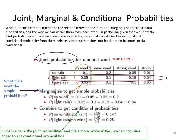
This table is the heart of our discussion today. Let's break down what it represents.

Joint Distribution

The four values in the center of the table represent the joint probability mass function (PMF), denoted as $p_{R,W}(r,w)=P(R=r,W=w)$. It tells us the probability of a specific pair of outcomes occurring simultaneously. For example, the probability of it being rainy and windy is $P(R=1,W=1)=0.02$. A joint distribution captures the complete probabilistic relationship between the variables.

Marginal Distribution

What if we only care about the probability of rain, regardless of the wind? We can get this by summing the joint probabilities over all possibilities for wind. This is called marginalization.

The marginal probability mass function for rain, $p_R(r)$, is found by summing the rows:

• $P(R=0)=p_{R,W}(0,0)+p_{R,W}(0,1)=0.58+0.1=0.68$
• $P(R=1)=p_{R,W}(1,0)+p_{R,W}(1,1)=0.3+0.02=0.32$

Notice that these sums are written in the "margin" of the table, which is where the name comes from. The marginal distribution $p_R(r)$ is the probability distribution of the random variable $R$ on its own.

Conditional Distribution

Finally, what if we want to know the probability of rain, given that we know it is windy? This brings us to the conditional probability mass function, $p_{R|W}(r|w)$, which is defined using the familiar rule for conditional probability:

$p_{R|W}(r|w)=P(R=r|W=w)=\frac{P(R=r,W=w)}{P(W=w)}=\frac{p_{R,W}(r,w)}{p_W(w)}$

For example, the probability of rain given that it's windy is:
$P(R=1|W=1)=\frac{p_{R,W}(1,1)}{p_W(1)}=\frac{0.02}{0.12}\approx 0.167$
This tells us that if you observe it's windy, the probability of it also being rainy is about 16.7%.

Test your understanding!

Using the table above, calculate the probability of it being windy given that there is no rain, i.e., $P(W=1|R=0)$.

Show answer

First, we identify the necessary probabilities from the table:

• The joint probability is $P(W=1,R=0)=p_{R,W}(0,1)=0.1$.
• The marginal probability is $P(R=0)=0.68$.

Now, we apply the definition of conditional probability:
$P(W=1|R=0)=\frac{P(W=1,R=0)}{P(R=0)}=\frac{0.1}{0.68}\approx 0.147$
So, there's about a 14.7% chance of it being windy if we know it's not raining.

2. Formal Definitions for Discrete and Continuous Variables

The intuitive ideas of joint, marginal, and conditional distributions apply to continuous variables as well, but we replace summations with integrals. The following document from Stanford's CS229 course provides the formal, rigorous definitions you'll need.

To summarize the key parallels between discrete and continuous cases:

Concept	Discrete Case (PMF)	Continuous Case (PDF)
Joint	$p_{X,Y}(x,y)=P(X=x,Y=y)$	$f_{X,Y}(x,y)$ where $P((X,Y)\in A)={\iint }_A{f}_{X,Y}(x,y)dxdy$
Marginal	$p_X(x)={\sum }_y{p}_{X,Y}(x,y)$	$f_X(x)={\int }_{-\infty }^{\infty }{f}_{X,Y}(x,y)dy$
Conditional	$ p_{Y	X}(y

3. A Deeper Dive: A Continuous Example

Let's apply these definitions to a more complex continuous problem. A common way to test understanding is with a uniform distribution over a non-rectangular region. This forces careful application of the integral definitions.

The following video from Harvard's Statistics 110 course works through an excellent example: finding the marginal and conditional PDFs for a point chosen uniformly at random from a disk of radius 1.

This example beautifully illustrates that even if the joint distribution is "uniform," the marginal distributions are not. The marginal PDF for $x$ is $f_X(x)=\frac{2}{\pi }\sqrt{1-x^2}$, which is highest at $x=0$ and zero at $x=\pm 1$. This should make intuitive sense: if you pick a random point in a disk, it's more likely to have an x-coordinate near the center than near the edge.

4. Generalization to Multiple Variables and the Chain Rule

These concepts extend naturally from two to $n$ random variables. A joint distribution can be defined over $X_1,X_2,\dots ,X_n$, and we can find the marginal distribution of any subset of these variables by integrating or summing out the others.

The definition of conditional probability leads to one of the most important formulas in probabilistic modeling: the chain rule of probability. Just as $P(A,B)=P(A|B)P(B)$, we can decompose a joint distribution into a product of conditional distributions. For three variables, this is:
$f(x,y,z)=f(x|y,z)f(y,z)=f(x|y,z)f(y|z)f(z)$

In general, for $n$ variables:
$f(x_1,\dots ,x_n)=f(x_1)f(x_2|x_1)f(x_3|x_1,x_2)\cdots f(x_n|x_1,\dots ,x_{n-1})=f(x_1){\prod }_{i=2}^{n}f(x_i|x_1,\dots ,x_{i-1})$

This rule allows us to build complex joint distributions from simpler conditional ones. This is the foundational principle behind Bayesian Networks and other graphical models you may have encountered in your AI studies. The following video explains this rule and also introduces the important related concept of conditional independence.

Conclusion

Today's lesson provided the essential vocabulary and mathematical tools for working with multiple random variables. While the concepts may seem abstract, they form the bedrock of how we model uncertainty in complex systems.

Key Takeaways:

• A joint distribution describes the simultaneous behavior of multiple random variables.
• A marginal distribution describes the behavior of a single variable, which is found by "marginalizing" (summing or integrating) out all other variables from the joint distribution.
• A conditional distribution describes the behavior of one variable given the known value of another, defined as the ratio of the joint to the marginal distribution.
• The chain rule allows us to decompose a complex joint distribution into a product of simpler conditional distributions, a cornerstone of probabilistic AI models.

Preview of the Next Lesson:
In this lesson, we focused on defining the concepts. In the next lesson, "Compute marginal and conditional distributions from a given joint distribution," we will put this theory into practice. You will work through concrete problems where you are given a joint PMF or PDF and must derive the corresponding marginal and conditional distributions yourself.