Quantum Monte Carlo for Interacting Systems

Hello! Welcome to the final lesson in our module on advanced computational methods.

In our previous lessons, we explored deterministic methods based on the Matrix Product State (MPS) ansatz, like DMRG and TEBD. You saw how incredibly effective they are for one-dimensional systems. However, their power diminishes rapidly in higher dimensions due to the unfavorable scaling of entanglement, a phenomenon known as the "area law" for generic ground states.

Today, we pivot to a completely different and powerful paradigm: Quantum Monte Carlo (QMC). These are stochastic methods that use random sampling to tackle problems that are intractable for deterministic approaches, especially in two or more dimensions.

Your learning outcome for this lesson is to outline the principles of Quantum Monte Carlo methods for interacting systems, focusing on Auxiliary-Field QMC (AFQMC) and Diagrammatic QMC (DiagMC). Instead of implementing an algorithm, our goal is to build a strong conceptual understanding of how these methods work, their underlying mathematical tricks, and their most significant challenge—the infamous fermion "sign problem".

1. The Core Idea: Monte Carlo for Quantum Systems

At its heart, Quantum Monte Carlo is a set of techniques for evaluating very high-dimensional integrals using random sampling. You're likely familiar with this from statistical mechanics, where properties are calculated by averaging over a Boltzmann distribution.

In quantum mechanics, the key is the imaginary-time propagator, $e^{-\beta \hat{H}}$. As you know, applying this operator to a trial state $|{\Psi }_T⟩$ and taking the limit $\beta \to \infty$ projects out the ground state $|{\Psi }_0⟩$. Observables can then be calculated as:

$$⟨\hat{O}⟩=\frac{⟨{\Psi }_0|\hat{O}|{\Psi }_0⟩}{⟨{\Psi }_0|{\Psi }_0⟩}=\underset{\beta \to \infty }{\lim }\frac{⟨{\Psi }_T|e^{-\beta \hat{H}/2}\hat{O}{e}^{-\beta \hat{H}/2}|{\Psi }_T⟩}{⟨{\Psi }_T|e^{-\beta \hat{H}}|{\Psi }_T⟩}$$

The denominator is analogous to a partition function, $Z=\text{Tr}(e^{-\beta \hat{H}})$, and the whole expression resembles a thermal expectation value at zero temperature.

Using the Trotter-Suzuki decomposition we saw in the last lesson, we can break the propagator into small time slices:

$$e^{-\beta \hat{H}}={\left(e^{-\Delta \tau \hat{H}}\right)}^N(\text{where }\beta =N\Delta \tau )$$

This expression is a quantum path integral in discrete imaginary time. The challenge is that for an interacting Hamiltonian $\hat{H}={\hat{H}}_1+{\hat{H}}_2$, the operator $e^{-\Delta \tau \hat{H}}$ is a complex many-body operator. QMC methods are ingenious ways of evaluating this path integral by sampling trajectories through the system's vast configuration space.

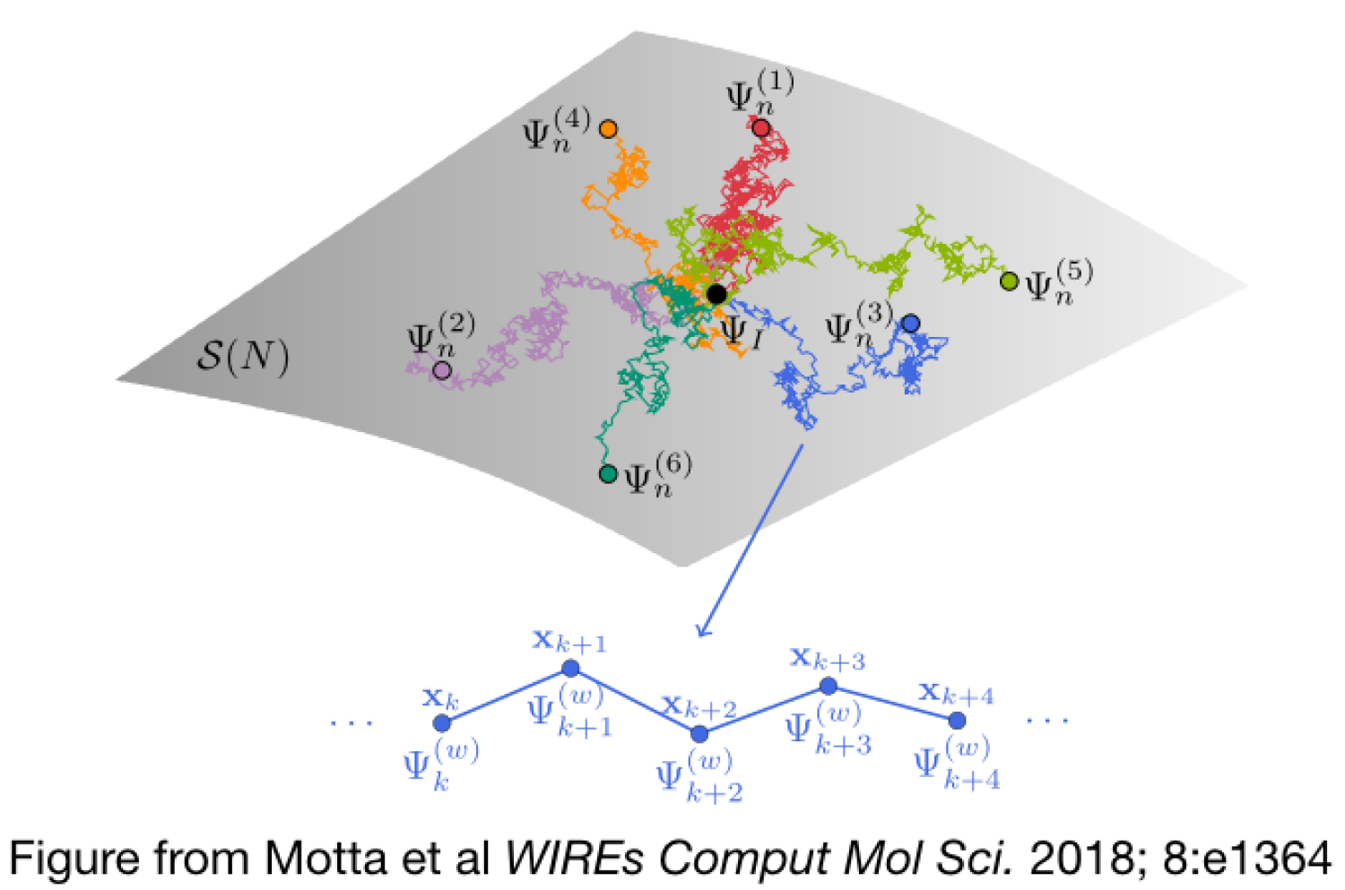
Different "flavors" of QMC arise from different ways of decomposing the propagator $e^{-\Delta \tau \hat{H}}$ and defining the space to be sampled. Let's explore two of the most important families for correlated systems.

2. Auxiliary-Field Quantum Monte Carlo (AFQMC)

AFQMC is a powerful method for fermionic systems like the Hubbard model or the electron gas, which are central to condensed matter physics. Its brilliance lies in a mathematical trick that converts an interacting problem into an average over many non-interacting problems.

The Hubbard-Stratonovich Transformation

The main difficulty in evaluating $e^{-\Delta \tau \hat{H}}$ comes from the two-body interaction term, ${\hat{H}}_2$. For example, in the Hubbard model, ${\hat{H}}_2=U{\sum }_i{n}_{i\uparrow }{n}_{i\downarrow }$. Since the $n_i$ operators are quadratic in fermion operators ($n_{i\sigma }=c_{i\sigma }^{†}{c}_{i\sigma }$), ${\hat{H}}_2$ is a four-fermion term.

The Hubbard-Stratonovich (HS) transformation is a way to exactly rewrite the exponential of a two-body operator as an integral over an exponential of a one-body operator, at the cost of introducing a new, random "auxiliary" field. Schematically, it looks like this:

$$e^{-\Delta \tau {\hat{v}}^2}=\frac{1}{\sqrt{2\pi }}{\int }_{-\infty }^{\infty }dx{e}^{-x^2/2}{e}^{\sqrt{-2\Delta \tau }x\hat{v}}$$

where $\hat{v}$ is a one-body operator. The key insight is that the complicated two-body interaction ${\hat{v}}^2$ on the left is replaced by a simple one-body operator $\hat{v}$ on the right, which is then averaged over all possible values of a random Gaussian variable $x$.

By applying this transformation, the propagator for one imaginary time step becomes a weighted average over propagators for non-interacting fermions moving in a fluctuating external field $\sigma$:

$$e^{-\Delta \tau \hat{H}}\approx \int d\sigma p(\sigma )\hat{B}(\sigma )$$

Here, $\hat{B}(\sigma )$ is a one-body propagator that depends on the specific configuration of the auxiliary field $\sigma$.

The full imaginary-time evolution becomes a path integral over trajectories of these auxiliary fields, $\sigma (\tau )$. At each step, the wavefunction can be represented by a single Slater determinant (since it's only ever evolved by one-body operators). The ground state is then a linear combination of all Slater determinants generated along these random paths.

The Fermion Sign Problem

This method seems perfect, but there's a profound difficulty. For fermions, the "weights" being sampled can be negative or complex. This is the notorious fermion sign problem.

In AFQMC, the weight of a particular path is related to the overlap of Slater determinants, $\det ({\Phi }_1^{†}{\Phi }_2)$, which can be negative. The Monte Carlo sampler therefore sums a series of large positive and negative numbers to find a small final answer. The statistical noise (variance) grows exponentially with the system size and inverse temperature ($\beta$), quickly overwhelming the signal. This is the single biggest obstacle to applying QMC to many interesting fermion problems.

Modern AFQMC methods control the sign problem using the constrained path or phaseless approximation. The idea is to use a known trial wavefunction, $|{\Psi }_T⟩$, to guide the random walk. Any walker (Slater determinant $|\varphi ⟩$) that tries to cross the nodal surface of the trial function (i.e., where $\text{Re}(⟨{\Psi }_T|\varphi ⟩)$ changes sign) is discarded. This makes the method approximate, with the quality of the result depending on the quality of the trial wavefunction's nodes. Fortunately, for many systems, even simple trial functions from mean-field theory yield remarkably accurate results.

3. Diagrammatic Monte Carlo (DiagMC)

DiagMC is a different, equally powerful QMC family. Instead of the HS transformation, DiagMC is based on stochastically summing a perturbative expansion to infinite order.

The Concept: Sampling Feynman Diagrams

Recall from your QFT course that physical quantities can be expressed as a diagrammatic expansion in powers of an interaction. For example, the partition function can be written as:

$$Z=\text{Tr}\left(e^{-\beta ({\hat{H}}_0+\hat{V})}\right)=\sum _{n=0}^{\infty }\frac{(-1{)}^n}{n!}{\int }_0^{\beta }\cdots {\int }_0^{\beta }d{\tau }_1\dots d{\tau }_n\text{Tr}\left(e^{-\beta {\hat{H}}_0}{T}_{\tau }[\hat{V}({\tau }_1)\dots \hat{V}({\tau }_n)]\right)$$

Each term in this sum corresponds to a set of Feynman diagrams of order $n$. DiagMC's central idea is to treat the space of all possible diagrams as the configuration space for a Monte Carlo simulation.

The algorithm performs a random walk in this abstract space of diagrams. The "moves" consist of:

• Increasing the diagram order (e.g., adding a vertex).
• Decreasing the diagram order (e.g., removing a vertex).
• Shifting the time coordinates of vertices.
• Other updates specific to the problem.

By sampling this space according to rules that satisfy detailed balance, the method can effectively sum the perturbation series to infinite order without ever truncating it.

Test your understanding!

Both AFQMC and DiagMC must tackle the evaluation of $e^{-\beta \hat{H}}$. In one sentence each, what is the core mathematical strategy each method uses to make the problem tractable for Monte Carlo sampling?

Show answer

• AFQMC: It uses the Hubbard-Stratonovich transformation to convert the interacting many-body problem into an average over non-interacting problems in fluctuating one-body auxiliary fields.
• DiagMC: It stochastically samples terms in a formal perturbation series of the partition function (or Green's function), effectively summing the series of all Feynman diagrams to infinite order.

Weak-Coupling vs. Strong-Coupling Flavors

Just as in standard perturbation theory, the choice of what you consider "small" and expand in is crucial. DiagMC methods for impurity models are often categorized by this choice:

• Weak-Coupling (CT-AUX): This method expands in powers of the on-site interaction U. It works well when U is small or for large clusters of atoms where electrons are more delocalized. This is conceptually similar to the AFQMC we discussed.
• Strong-Coupling (CT-HYB): This method expands in powers of the hybridization V between the impurity and the surrounding bath. It is exceptionally powerful for strongly correlated problems where U is large, as the average order of the diagrams being sampled actually decreases with U. This is the workhorse solver in many Dynamical Mean-Field Theory (DMFT) studies.

These two approaches are complementary, each excelling in a different physical regime. The choice of which to use depends on the specific problem you are trying to solve.

Conclusion

In this lesson, we have surveyed the principles of Quantum Monte Carlo methods, a vast and powerful toolkit for many-body physics. Unlike the deterministic tensor network methods from the last lessons, QMC uses stochastic sampling to navigate the immense Hilbert spaces of quantum systems.

Key Takeaways:

• QMC methods formulate quantum problems, like finding a ground state via imaginary-time projection, as high-dimensional integrals that can be evaluated by random sampling.
• Auxiliary-Field QMC (AFQMC) uses the Hubbard-Stratonovich transformation to linearize the interaction, recasting the problem as an average over non-interacting systems in random fields. Its walkers are Slater determinants.
• Diagrammatic QMC (DiagMC) performs a random walk in the space of Feynman diagrams, stochastically summing a perturbation series to infinite order.
• The fermion sign problem, where negative or complex weights lead to exponential decay of the signal-to-noise ratio, is the primary obstacle for fermionic QMC. It is often managed with approximations like the constrained-path method, which turn a potentially exact method into a highly accurate, approximate one.

Preview of the Next Module:
Our discussion of QMC, particularly DiagMC, provides a perfect bridge to our next major topic. Many of these algorithms are designed to compute a central quantity in many-body theory: the single-particle Green's function. In the next module, Diagrammatic Many-Body Perturbation Theory, we will leave the world of numerical algorithms behind for a while and dive deep into the analytical theory of Green's functions. We will define them, explore their physical meaning, and learn how to calculate them using the very Feynman diagrams that DiagMC so cleverly samples.