Combinatorial Strategy: Backtracking vs. Dynamic Programming

Welcome back! In our previous lesson, we developed a framework for selecting the right graph algorithm by analyzing the problem's structure and goals. This approach of moving from ambiguity to a clear plan is central to mastering algorithmic problem-solving.

We're now in the final, most challenging module of the course, where the goal is to synthesize everything you've learned. Today, we'll extend that same "choose the right tool" mindset to a different class of problems: combinatorial search. You'll often encounter problems that ask you to find arrangements, subsets, or combinations that satisfy a set of rules. These usually boil down to a choice between two powerful techniques: Backtracking and Dynamic Programming (DP).

This lesson is designed to help you solve an unseen Medium combinatorial problem by confidently choosing between these two approaches. We will establish a clear decision framework and define the "state" that each technique requires you to track.

The Fundamental Divide: Exploration vs. Optimization

At their core, Backtracking and Dynamic Programming both explore a large space of possibilities. However, they are used for fundamentally different purposes.

• Backtracking is a tool for exploration and enumeration. Its goal is to systematically search through all possible candidates. It's like exploring every path in a maze, but with the intelligence to turn back ("backtrack") the moment you realize a path is a dead end. Use it when you need to generate all valid solutions.

• Dynamic Programming is a tool for optimization and counting. It's a "brute-force with a memory." It breaks a problem into overlapping subproblems, solves each subproblem just once, and stores the result to avoid redundant work. Use it when you need to find the one best solution (minimum, maximum) or count the total number of ways to do something.

To build a solid intuition for this distinction, we'll start with a great video that introduces the core idea of backtracking as a decision tree.

A Framework for Choosing

The most common source of confusion is knowing when to apply which technique. Here is a simple decision process:

1. Analyze the Goal: Read the problem statement carefully. What is it asking for?

   • If it contains phrases like "find all possible...", "generate all combinations/permutations", or "all valid arrangements", your first thought should be Backtracking.
   • If it contains phrases like "optimal", "minimum cost", "maximum profit", "longest/shortest", or "count the number of ways", your first thought should be Dynamic Programming.

2. Analyze the Structure:

   • For Backtracking, the problem typically involves making a sequence of choices under a set of constraints. The state is the partial solution you've built so far.
   • For Dynamic Programming, the problem must exhibit two properties:
     • Optimal Substructure: The optimal solution to the overall problem can be constructed from the optimal solutions of its subproblems.
     • Overlapping Subproblems: The same subproblems are solved many times over in a naive recursive approach.

This distinction is crucial and worth exploring visually. The following video explains the two core properties of DP problems.

The article "Master Dynamic Programming, BFS & Backtracking" provides an excellent written summary of these patterns, along with helpful JavaScript templates.

Deep Dive 1: Backtracking State and Pruning

When you choose backtracking, your main task is to define the state for the recursive function and the constraints for pruning. The state typically includes:

1. The partial solution being built (e.g., currentPath, currentBoard).
2. Parameters to track progress and available choices (e.g., currentIndex, currentRow).

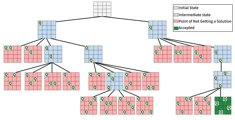
The canonical example is the N-Queens puzzle: place N queens on an N×N board so none attack each other.

• Goal: Find all valid board configurations. This is a clear signal for backtracking.
• State: The placement of queens in the rows processed so far. We can represent this as an array where placement[row] = col.
• Choices: For each row, we can try placing a queen in any of the N columns.
• Constraints (Pruning): We cannot place a queen in a column or diagonal that is already attacked. We prune any branch of the search tree that attempts this.

This image beautifully illustrates the state-space tree that backtracking explores for N-Queens. The red nodes are branches that were pruned because they violated a constraint.

Let's see how this translates into a universal template that you can adapt for many problems.

Deep Dive 2: Dynamic Programming State and Transitions

When you choose DP, the most critical step is defining the state. The state, often dp[i] or dp[i][j], encapsulates the solution to a subproblem.

• dp array/table: This stores the solutions to the subproblems.
• State Definition: dp[i] means "the optimal solution/count for the problem of size i". For example, dp[i] could be "the minimum cost to reach step i" or "the number of ways to make change for amount i".
• Transition (Recurrence Relation): This is the formula that computes dp[i] using previously computed values (e.g., dp[i-1], dp[i-2]).
• Base Cases: The smallest subproblems that can be solved directly.

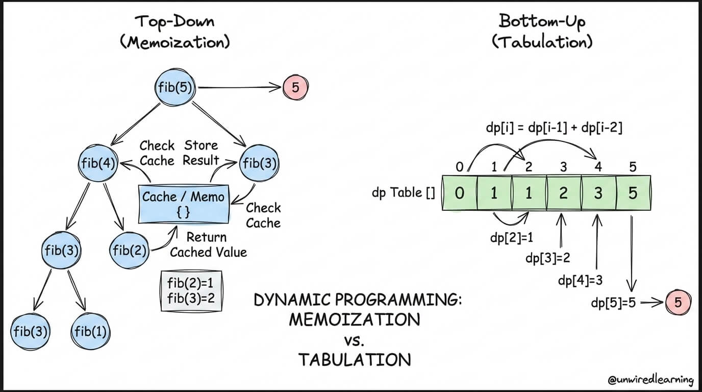
The image below contrasts the two main flavors of DP: Memoization (top-down, recursive) and Tabulation (bottom-up, iterative). You can think of memoization as a recursive backtracking-style solution that caches its results. Tabulation builds the solution from the ground up.

Let's apply this to a classic problem: Coin Change (LeetCode 322). Given coins = [1, 2, 5] and amount = 11, find the minimum number of coins to make the amount.

1. Goal: "minimum number" -> DP.
2. Could we use Backtracking? Yes, we could find all combinations that sum to 11 and pick the shortest. But we'd re-calculate the subproblem "min coins for amount 6" many times.
3. DP Approach:
   • State: Let dp[i] be the minimum number of coins to make amount i.
   • Base Case: dp[0] = 0 (0 coins for amount 0).
   • Transition: To find dp[i], we can try using any of our available coins. If we use a coin c, we are left with the subproblem of making amount i - c. The number of coins for this choice would be dp[i - c] + 1. Since we want the minimum, we take the minimum over all possible coin choices. $$dp[i]=\underset{c\in \text{coins}}{\min }(dp[i-c]+1)$$
   • Final Answer: dp[amount], which is dp[11].

The tabulation approach would be to create an array dp of size 12, initialize dp[0] = 0, and fill the rest of the array with infinity. Then, iterate from i = 1 to 11, applying the transition formula at each step.

Summary and Key Takeaways

You now have a powerful framework for tackling a huge category of interview problems. When faced with a combinatorial search problem:

• First, ask: What is the goal?

  • "Find all solutions" or "generate all permutations/combinations" → Backtracking.
  • "Find the optimal (min/max) value" or "count the ways" → Dynamic Programming.

• If it's Backtracking:

  • Think in terms of a decision tree.
  • Use the choose-explore-unchoose template.
  • Define the state passed to your recursive function.
  • Identify the constraints that allow you to prune the search.

• If it's Dynamic Programming:

  • Confirm it has optimal substructure and overlapping subproblems.
  • Clearly define the meaning of your DP state (e.g., dp[i] = ...).
  • Find the transition formula (recurrence relation) that builds larger solutions from smaller ones.
  • Establish the base cases.

This structured thinking process is your best defense against "algo phobia." It turns a guess into a logical deduction.

In our next lesson, we will focus on another critical interview skill: repairing a flawed solution. You'll be given broken code and asked to locate the error—a task that requires the same deep pattern-recognition skills we've developed today.