Wavelet Decomposition for Multi-Scale Feature Engineering

In our previous lesson, we delved into measuring the magnitude of market turbulence by engineering volatility features using GARCH models and realized volatility. We learned to quantify risk by looking at how much a time series fluctuates. Today, we will approach our signal from an entirely different and powerful perspective. Instead of just measuring the size of changes, we'll learn to decompose the signal itself into its fundamental building blocks, operating at different frequencies and at different moments in time.

This lesson introduces the wavelet transform, a mathematical tool that acts like a microscope for time series data. It allows us to see not only what frequencies are present in a signal (like short-term noise or long-term trends) but also precisely when they occur. For financial data, where market dynamics are non-stationary and events unfold across multiple time horizons, this is an exceptionally powerful capability. You'll learn how to apply these transforms and, most importantly, how to turn their output into highly informative features for your machine learning models.

The Limitation of a Frequency-Only View

Many signal processing techniques, such as the Fourier Transform, are designed to identify the frequency components of a signal. They answer the question: "What are the underlying rhythms or cycles in my data?" However, they do so at a cost: they lose all information about time.

To build a strong intuition for this limitation and to understand why wavelets are so revolutionary, let's start with a superb conceptual video.

As the video highlights, financial time series are like the traffic light signal: the "frequencies" (market dynamics) are not constant. A high-frequency, noisy period might be followed by a calm, low-frequency trend. A Fourier Transform would average this out, but a wavelet transform can pinpoint each regime in both time and frequency.

The Wavelet: A Time-Frequency Microscope

The wavelet transform overcomes the limitations of the Fourier transform by using a different kind of analyzing function. Instead of the infinitely long sine and cosine waves, it uses a wavelet—a small, localized wave-like oscillation that has a beginning and an end. The name itself, from French, literally means "little wave."

The core idea of the wavelet transform is to take this "mother wavelet" and do two things:

1. Scale it: Stretch it out to look for low-frequency phenomena and compress it to look for high-frequency events.
2. Translate it: Slide it along the signal's time axis to see where these frequency events are located.

At each time point and for each scale, we measure how well the wavelet matches the signal. This measurement is essentially a convolution, or a sliding dot product. A high value means the signal has significant energy at that specific time and scale (frequency).

The following segment from the "Wavelets: a mathematical microscope" video provides an excellent visualization of this entire process.

The Scalogram: Visualizing Time and Frequency

The result of performing a Continuous Wavelet Transform (CWT) is a set of coefficients for every point in time and for every scale. We can visualize these coefficients as a 2D plot called a scalogram or time-frequency heatmap.

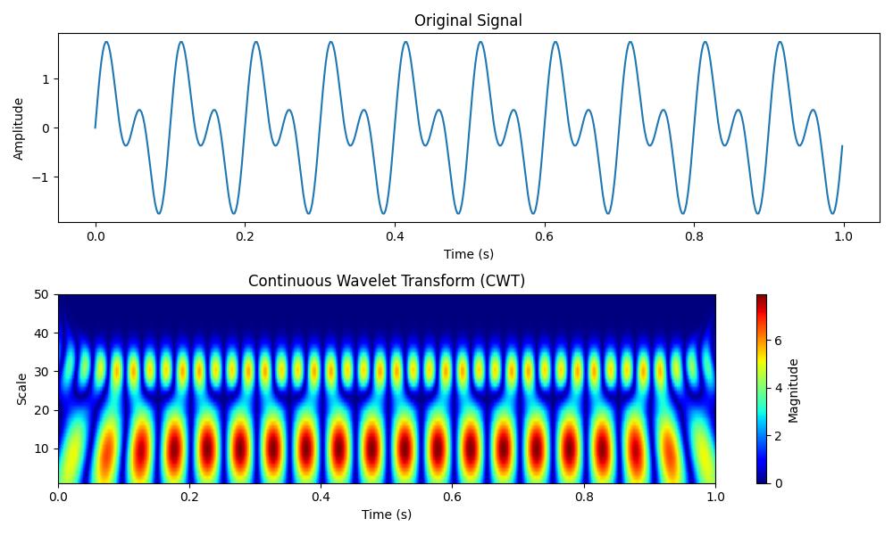
In this scalogram, you can clearly see how the signal's frequency content changes over time. The bright yellow bands at the bottom represent high-energy, high-frequency (low scale) oscillations that are persistent throughout the signal. This ability to resolve a signal in both time and frequency is what makes the wavelet transform so powerful for feature engineering.

From Transform to Features

Now for the crucial step: how do we convert these wavelet coefficients into features a machine learning model can use? There are two primary strategies, both of which are very powerful.

Strategy 1: The Scalogram as an Image for CNNs

This is a particularly elegant approach that leverages your background in computer vision. The 2D scalogram is, for all intents and purposes, an image. It's a 2D representation of a 1D time series. You can generate a scalogram for each time series instance in your dataset and use these images to train a Convolutional Neural Network (CNN).

The CNN will learn to detect patterns in the scalogram—such as specific shapes, textures, or localized bright spots—that are predictive of the target variable. This method automates the process of feature extraction from the time-frequency domain.

To see a practical application of this, let's look at a blog post that uses this exact technique for classifying ECG signals.

Strategy 2: Statistical Features from Decomposition Levels

A more traditional, but still highly effective, approach is to extract statistical features from the wavelet coefficients at each scale. The wavelet transform decomposes the original signal into several new time series, one for each scale, representing different frequency bands (e.g., short-term details, medium-term components, long-term trends).

From each of these new time series (sub-bands), you can compute a battery of statistical features, such as:

• Mean
• Variance / Standard Deviation
• Skewness / Kurtosis
• Energy ($\sum C_i^2$, where $C_i$ are the coefficients)
• Entropy (a measure of complexity)

This process converts a single time series into a rich set of tabular features that can be used by any standard machine learning model like Gradient Boosting or a simple MLP.

Practical Implementation in Python

Implementing the CWT and generating scalograms in Python is straightforward with the PyWavelets library. The following video tutorial walks through the necessary code.

Interview Alert: You are tasked with building a model to predict stock market crashes from price data. A colleague suggests using standard time-series features like moving averages and momentum. How could you propose a more advanced feature set to capture multi-scale dynamics that might precede a crash?

A top-tier response would be: "In addition to standard features, I would use a wavelet transform to create a multi-scale representation of the price series. Market dynamics leading to a crash often involve interactions across different time horizons—for example, a breakdown of a long-term trend combined with a spike in short-term volatility.

I would implement this in two ways. First, I would generate scalograms from the return series over, say, the last year of data. These 2D images, which capture the full time-frequency landscape, would be fed into a CNN. This allows the model to learn complex, non-linear patterns that are indicative of an impending crash.

Second, to complement the CNN, I'd use a Discrete Wavelet Transform (DWT) to decompose the signal into several frequency bands. From each band, I would extract statistical features like variance, energy, and entropy. This creates a set of tabular features that explicitly quantify the behavior at different scales (e.g., 'volatility of the 2-4 day component', 'energy of the 16-32 day component'), which could then be fed into a Gradient Boosting model alongside the standard features."

Conclusion

Today, we've unlocked a new dimension in time series analysis. By moving beyond the time domain and into the joint time-frequency domain, we can create features that capture a far richer picture of a signal's dynamics.

Key Takeaways:

• Time-Frequency Localization: Unlike the Fourier Transform, which loses all time information, the wavelet transform tells you both what frequencies are in a signal and when they occur.
• Ideal for Non-Stationary Data: This property makes wavelets perfectly suited for analyzing financial time series, where volatility, trends, and cycles evolve over time.
• The Scalogram: The output of a CWT is a 2D matrix of coefficients that can be visualized as a scalogram, providing an intuitive map of the signal's energy across time and frequency.
• Multi-Scale Feature Creation: You can engineer features either by treating the scalogram as an image for a CNN or by computing statistical summaries on the different frequency sub-bands produced by the transform.

In our lessons so far, we have focused on extracting features from a single time series. In our next session, we will expand our view to engineer features that capture the relationships between multiple time series, such as correlations, spreads, and lead-lag effects—a critical skill for building robust financial models.