Neural Network Learning: Backpropagation and Loss Functions

Hello! Let's dive into the second lesson of our course.

In our last lesson, we established that a neural network is essentially a very complex function with a vast number of tunable parameters—the weights and biases. We saw how data flows forward through layers of neurons, with each neuron performing a simple calculation.

Today, we'll answer the most important question: How does the network "learn" the correct values for those millions of parameters? This lesson addresses the learning outcome: Describe how neural networks learn by minimizing a loss function via backpropagation at a conceptual level.

We'll break this "learning" process down into three core ideas:

1. Loss Function: A way to score the network's performance, telling it how wrong its predictions are.
2. Gradient Descent: An optimization algorithm that uses the score to iteratively "nudge" the network's parameters in the right direction.
3. Backpropagation: The engine that efficiently calculates how to perform those nudges for every parameter in the network.

1. Quantifying Error: The Loss Function

Before a network can improve, it needs a way to measure its own error. A loss function (also called a cost function) does exactly this. It takes the network's predictions and the true labels and boils them down to a single number representing the "lousiness" of the predictions. The higher the number, the worse the network is performing. The goal of training is to make this number as small as possible.

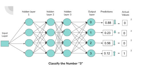
Let's return to the handwritten digit example. If we feed the network an image of a '3', the ideal output would be a '1' at the third output neuron and '0' for all others. A poorly trained network might output random-looking values.

To see how we quantify this error, let's watch the first part of the next video from 3Blue1Brown.

As the video explains, a common approach is to calculate the sum of squared errors. For each of the 10 output neurons, you find the difference between its activation value and the target value (0 or 1), square that difference, and then add up these squared differences. The total sum is the loss for that single training example.

When you average this loss across thousands of training examples, you get a single number that measures the overall performance of the network for its current set of weights and biases.

2. Finding the Minimum: Gradient Descent

So, we have a loss function that depends on thousands of parameters (weights and biases). You can imagine this as a vast, high-dimensional landscape. Our goal is to find the lowest point in this landscape—the combination of parameters that results in the minimum loss.

The algorithm for finding this minimum is called gradient descent.

Imagine you're standing on a hillside in a thick fog. You want to get to the bottom of the valley, but you can only see the ground at your feet. The best strategy is to feel which direction is steepest downhill and take a small step in that direction. Repeat this process, and you'll eventually find your way to the bottom.

This is the intuition behind gradient descent:

• The "slope" in any direction is given by the gradient of the loss function. The gradient is a vector that points in the direction of the steepest ascent.
• Therefore, to go downhill, we take a step in the direction of the negative gradient.
• The "size" of the step we take is called the learning rate.

Let's continue with the 3Blue1Brown video, which visualizes this process beautifully.

To make this more interactive, let's explore a hands-on explainer.

The process seems straightforward: calculate the gradient and take a step. But how do we calculate the gradient for a function with thousands or millions of inputs (our weights and biases)? Calculating it by "wiggling" each parameter one by one would be computationally impossible. This is where backpropagation comes in.

3. The Engine of Learning: Backpropagation

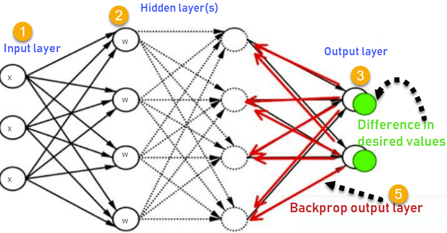
Backpropagation is a remarkably efficient algorithm for calculating the gradient of the loss function with respect to every single weight and bias in the network. Its name, "backward propagation of errors," hints at how it works.

Here's the conceptual flow:

1. Forward Pass: A training example is fed through the network, and we calculate the output.
2. Calculate Error: The loss function measures the error at the output layer.
3. Backward Pass: The algorithm starts at the output layer and works its way backward. At each neuron, it calculates how much that neuron contributed to the error in the layer ahead of it. This "error contribution" signal is then passed back to the preceding layer.

This backward flow allows the algorithm to determine how sensitive the final loss is to each weight and bias. A weight that has a large impact on the final error will get a large gradient value, signaling that it needs a significant adjustment.

This is made possible by the chain rule from calculus. Conceptually, if a change in weight w affects neuron B, and neuron B affects the final loss C, the chain rule lets us calculate the total effect of w on C by multiplying the individual effects.

The 3Blue1Brown channel has another superb video explaining this intuitively.

4. The Full Training Loop

Now let's assemble these pieces into the complete training process, which from your software engineering background you can think of as a training loop.

1. Initialization: The network's weights and biases are initialized with small random values.
2. Iteration (Looping through Epochs): The network iterates over the training data multiple times. Each full pass over the dataset is called an epoch.
3. Inside the loop, for each batch of data:
   a. Forward Pass: Make predictions for the current batch of data.
   b. Compute Loss: Use the loss function to calculate the error for the batch.
   c. Backward Pass (Backpropagation): Compute the gradient of the loss with respect to all parameters.
   d. Update Parameters (Gradient Descent): Nudge all weights and biases in the opposite direction of the gradient, scaled by the learning rate.

A practical detail mentioned in the video is the use of mini-batches. Calculating the true gradient requires averaging the error over the entire dataset, which is very slow. Instead, we use a small, random subset of the data (a "mini-batch," e.g., 32-256 examples) to get a noisy but fast approximation of the gradient. This method is called Stochastic Gradient Descent (SGD). It's like the "drunken man stumbling downhill" — less precise at each step, but much faster overall.

Conclusion

In this lesson, we've demystified how a neural network "learns." It's not magic, but a powerful optimization process.

Key Takeaways:

• Learning is Optimization: The goal of training is to find the set of weights and biases that minimizes a loss function.
• Loss Function: This function scores the network's performance by measuring the difference between its predictions and the actual target values.
• Gradient Descent: This is the iterative algorithm used to find the minimum of the loss function. It involves taking small steps in the direction of the negative gradient (the direction of steepest descent).
• Backpropagation: This is the core algorithm that makes learning feasible. It efficiently calculates the gradient for all network parameters by propagating error information backward from the output layer, using the chain rule.

We now have a complete, albeit conceptual, picture of how a basic neural network works and learns. However, the simple architecture we've seen so far isn't well-suited for processing sequential data like language.

In our next lesson, we will begin our journey toward modern language models by tackling the first challenge: how to convert text into a numerical format that a neural network can understand. We'll explore the concepts of tokens and token embeddings.