Feynman Path Integral from the Propagator

Hello! Welcome to the first lesson of our new module on the Feynman Path Integral.

In our previous modules, we developed a powerful understanding of quantum mechanics through the operator formalism, culminating in a generalized description of open systems and measurement. We now pivot to a completely different, yet fully equivalent, formulation of quantum theory. Instead of states evolving via operators, we will consider the quantum amplitude for a particle to travel between two points as a sum over all possible trajectories, or "histories," connecting them.

This path integral approach, pioneered by Richard Feynman, offers profound physical intuition, especially regarding the emergence of classical mechanics. It also provides a direct link between quantum mechanics and statistical mechanics and serves as the foundation for modern quantum field theory. Your interest in condensed matter and many-body systems will be well-served by this perspective, as path integrals are a central tool in those fields.

Today, our goal is to answer the fundamental question: where does this radical idea come from? We will derive the Feynman path integral from the quantum mechanical propagator, starting from the familiar territory of the Schrödinger equation and its time-evolution operator.

1. The Intuitive Leap: From Two Slits to Infinite Paths

The conceptual seed of the path integral lies in the double-slit experiment. The interference pattern arises because we must sum the probability amplitudes for the particle to pass through each of the two slits. The total amplitude is $\Phi ={\Phi }_1+{\Phi }_2$.

Feynman's insight was to take this principle of superposition to its logical extreme. What if, instead of a screen with two slits, we had multiple screens with many slits? The amplitude would be the sum over all possible multi-segment paths. In the limit of an infinite number of screens placed infinitesimally close together, we are no longer summing over a discrete set of paths but integrating over a continuum of all possible trajectories a particle could take through spacetime.

To build this intuition, let's start with a reading that follows this exact line of reasoning.

This idea of summing over all paths, each contributing with a certain phase, is the heart of the path integral. The central object that we will formalize this with is the propagator.

2. The Propagator: The Starting Point for Our Derivation

In the Schrödinger picture, the evolution of a state $|\psi ⟩$ from time $t_i$ to $t_f$ is governed by the time-evolution operator $U(t_f,t_i)$. The propagator, often denoted $K$, is simply the representation of this operator in the position basis.

It is defined as the transition amplitude:

$$K(x_f,t_f;x_i,t_i)=⟨x_f|U(t_f,t_i)|x_i⟩$$

In words, the propagator is the probability amplitude for a particle that is at position $x_i$ at time $t_i$ to be found at position $x_f$ at time $t_f$. As you saw in the previous reading and in your study of Green's functions, knowing the propagator allows you to determine the wavefunction at any time $t_f$ given the wavefunction at an initial time $t_i$:

$$\psi (x_f,t_f)=\int d{x}_{i}K(x_f,t_f;x_i,t_i)\psi (x_i,t_i)$$

Our entire derivation will consist of finding an alternative expression for this propagator, $K(x_f,t_f;x_i,t_i)$.

3. The Derivation: From Operators to a Sum Over Histories

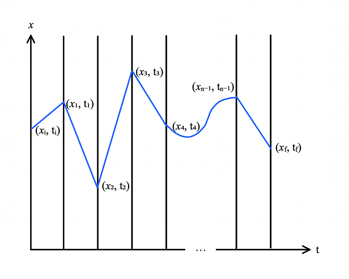
Our goal is to transform the operator expression $⟨x_f|e^{-iH(t_f-t_i)/\hslash }|x_i⟩$ into a sum over paths. The key technique is known as time slicing. We will break the total time interval $t=t_f-t_i$ into a large number, $N$, of infinitesimal steps of duration $ϵ=t/N$.

The following video provides a detailed, step-by-step derivation. I will break it down into four stages, with explanations to guide you.

Stage 1: Discretizing Time and Inserting Intermediate States

First, we write the time evolution operator as a product of $N$ short-time evolution operators:

$$U(t)=e^{-iHt/\hslash }={\left(e^{-iHϵ/\hslash }\right)}^N$$

The propagator then becomes:

$$K(x_f,t;x_i,0)=⟨x_f|\underset{N\text{ times}}{\underbrace{e^{-iHϵ/\hslash }\cdot e^{-iHϵ/\hslash }\cdots e^{-iHϵ/\hslash }}}|x_i⟩$$

Now, we insert a completeness relation, $\int d{x}_j|x_j⟩⟨x_j|=1$, between each of these short-time operators. This gives us:

$$K(x_f,t;x_i,0)=\int d{x}_1\cdots d{x}_{N-1}⟨x_f|e^{-iHϵ/\hslash }|x_{N-1}⟩⟨x_{N-1}|\cdots |x_1⟩⟨x_1|e^{-iHϵ/\hslash }|x_i⟩$$

We have transformed the problem of finding one propagator for the full time $t$ into finding $N$ propagators for the infinitesimal time $ϵ$ and then integrating over all intermediate positions. This sequence of points $(x_i,x_1,\dots ,x_{N-1},x_f)$ forms a discretized path in spacetime.

Stage 2: Evaluating the Infinitesimal Propagator

The core of the problem is now to evaluate the infinitesimal propagator $⟨x_{j+1}|e^{-iHϵ/\hslash }|x_j⟩$. For a Hamiltonian $H=T+V=\frac{{\hat{p}}^2}{2m}+V(\hat{x})$, the kinetic and potential energy operators do not commute. This means $e^{-i(T+V)ϵ/\hslash }\ne e^{-iTϵ/\hslash }{e}^{-iVϵ/\hslash }$.

However, for infinitesimal $ϵ$, we can use the first-order Trotter-Suzuki formula:

$$e^{-i(T+V)ϵ/\hslash }=e^{-iTϵ/\hslash }{e}^{-iVϵ/\hslash }+O({ϵ}^2)$$

In the limit $ϵ\to 0$, we can neglect the higher-order terms. Our infinitesimal propagator becomes:

$$⟨x_{j+1}|e^{-iTϵ/\hslash }{e}^{-iVϵ/\hslash }|x_j⟩$$

Since $|x_j⟩$ is an eigenstate of the potential operator $\hat{V}=V(\hat{x})$, we can simplify this to:

$$e^{-iV(x_j)ϵ/\hslash }⟨x_{j+1}|e^{-i{\hat{p}}^2ϵ/2m\hslash }|x_j⟩$$

To evaluate the remaining matrix element with the kinetic energy operator, we insert a completeness relation for the momentum basis, $\int \frac{dp}{2\pi \hslash }|p⟩⟨p|=1$. The first segment of the video (00:00 - 08:00) walks through this calculation in detail. The key steps are:

1. Expressing the matrix element $⟨x|p⟩$ as a plane wave $e^{ipx/\hslash }$.
2. Inserting the momentum basis to evaluate the matrix elements of $T$ and $V$.

Stage 3: Performing the Momentum Integral

After inserting the momentum basis, the infinitesimal propagator becomes a Gaussian integral over momentum $p$.

$$⟨x_{j+1}|e^{-iHϵ/\hslash }|x_j⟩\approx \int \frac{dp}{2\pi \hslash }{e}^{ip(x_{j+1}-x_j)/\hslash }\exp \left[-\frac{iϵ}{\hslash }\left(\frac{p^2}{2m}+V(x_j)\right)\right]$$

This integral can be solved by completing the square. The second and third segments of the video (08:00 - 14:27) show this calculation. The result is:

$$⟨x_{j+1}|e^{-iHϵ/\hslash }|x_j⟩\approx \sqrt{\frac{m}{2\pi i\hslash ϵ}}\exp \left\{\frac{iϵ}{\hslash }\left[\frac{m}{2}{\left(\frac{x_{j+1}-x_j}{ϵ}\right)}^2-V(x_j)\right]\right\}$$

Notice something remarkable here. The term in the exponent is precisely the classical Lagrangian, $L=T-V$, evaluated for the straight-line segment from $x_j$ to $x_{j+1}$, multiplied by the time step $ϵ$. This is the action for that infinitesimal path segment.

Stage 4: The Continuum Limit

Finally, we substitute this result back into our expression for the full propagator. This involves taking a product of $N$ such terms. The product of exponentials becomes the exponential of a sum:

$$K(x_f,t;x_i,0)=\underset{N\to \infty }{\lim }{\left(\frac{m}{2\pi i\hslash ϵ}\right)}^{N/2}\int d{x}_1\cdots d{x}_{N-1}\exp \left\{\frac{i}{\hslash }\sum _{j=0}^{N-1}ϵ\left[\frac{m}{2}{\left(\frac{x_{j+1}-x_j}{ϵ}\right)}^2-V(x_j)\right]\right\}$$

In the continuum limit as $N\to \infty$ and $ϵ\to 0$:

• The sum ${\sum }_{j=0}^{N-1}ϵL(x_j,{\dot{x}}_j)$ becomes a time integral of the Lagrangian, which is the classical action $S[x(t)]$:
  ${\sum }_{j=0}^{N-1}ϵL_j⟶{\int }_0^{t}L(x(\tau ),\dot{x}(\tau ))d\tau =S[x(t)]$
• The product of integrals over all intermediate points, together with the normalization factor, is formally defined as the path integral measure $\mathcal{D}[x(t)]$.
  ${\lim }_{N\to \infty }{\left(\frac{m}{2\pi i\hslash ϵ}\right)}^{N/2}\int d{x}_1\cdots d{x}_{N-1}⟶\int \mathcal{D}[x(t)]$

The final segment of the video (14:27 - 16:00) puts all these pieces together. The grand result is the Feynman Path Integral:

$$K(x_f,t_f;x_i,t_i)=\int \mathcal{D}[x(t)]e^{iS[x(t)]/\hslash }$$

This elegant formula states that the amplitude to go from an initial to a final point is the sum over all possible paths connecting them, where each path is weighted by a phase factor determined by its classical action.

Test your understanding!

In the derivation, we made the approximation $e^{-iHϵ/\hslash }\approx e^{-iTϵ/\hslash }{e}^{-iVϵ/\hslash }$. Why is this approximation justified in the limit $ϵ\to 0$, and what is the physical interpretation of the terms that are being neglected?

Show answer

This approximation is justified because the difference between the two expressions is of order ${ϵ}^2$. Specifically, the Baker-Campbell-Hausdorff formula tells us that $e^{A+B}=e^A{e}^B{e}^{-\frac{1}{2}[A,B]}\cdots$.
For $A=-iTϵ/\hslash$ and $B=-iVϵ/\hslash$, the leading correction term involves the commutator $[T,V]$ multiplied by ${ϵ}^2$.
So, for a single time slice, the error is $O({ϵ}^2)$. When we multiply $N=t/ϵ$ such terms together, the total accumulated error is of order $N\times {ϵ}^2=(t/ϵ){ϵ}^2=tϵ$. As we take the limit $ϵ\to 0$, this total error vanishes.

Physically, the commutator $[\hat{T},\hat{V}]=[\frac{{\hat{p}}^2}{2m},V(\hat{x})]$ represents the fact that a particle's kinetic and potential energies cannot be specified simultaneously with arbitrary precision. Neglecting the commutator term in each infinitesimal slice is equivalent to assuming that over an infinitesimally short time, the particle's position (affecting V) and momentum (affecting T) can be treated as momentarily definite. The path integral formalism correctly rebuilds the full quantum uncertainty by integrating over all possible values of these variables at all intermediate times.

Conclusion

In this lesson, we have bridged the gap between the familiar operator formalism and the path integral picture. By starting with the definition of the quantum propagator and applying the technique of time-slicing, we successfully derived Feynman's celebrated formula.

Key Takeaways:

• The quantum propagator $K(x_f,t_f;x_i,t_i)$ can be expressed as a sum over all possible paths connecting the initial and final spacetime points.
• The derivation hinges on discretizing the time evolution, inserting completeness relations at each time slice, and approximating the short-time evolution operator.
• Each path $x(t)$ contributes to the total amplitude with a complex weight $e^{iS[x(t)]/\hslash }$, where $S[x(t)]$ is the classical action for that path.
• This formulation brings the classical Lagrangian and the principle of least action to the forefront of quantum mechanics. Paths where the action is stationary (i.e., the classical path) interfere constructively, while paths far from it tend to have rapidly varying phases and interfere destructively, providing a beautiful explanation for the emergence of a single classical trajectory in the macroscopic limit.

Preview of the Next Lesson:
We have derived a beautiful and profound formula. But can we actually calculate anything with it? In the next lesson, we will put the path integral to work. We will learn how to calculate path integrals for a free particle and for the quantum harmonic oscillator analytically. These examples will not only solidify your understanding of the formalism but also demonstrate its power in solving canonical problems in quantum mechanics.