Activation Checkpointing: Trading Compute for Memory

Introduction

Welcome to the next lesson in our module on memory optimization. In our previous lesson, we explored how frameworks like DeepSpeed and PyTorch FSDP implement full model state sharding. This technique partitions the parameters, gradients, and optimizer states across multiple GPUs, allowing us to train models far larger than what could fit on a single device. We concluded that while this dramatically reduces the memory footprint of the model, another major consumer of GPU memory remains: activations.

Today, we address that challenge directly. This lesson will explain activation checkpointing (also known as gradient checkpointing), a powerful technique that drastically reduces activation memory by trading it for a modest amount of additional computation. You will learn the core mechanism behind this trade-off, explore different strategies from the theoretically optimal to the practically implemented, and understand the critical system-level implications for performance and stability.

This topic is fundamental to designing systems for training state-of-the-art models, where memory capacity is almost always a primary constraint.

1. The Activation Memory Problem

To execute the backward pass and compute gradients, the autograd engine needs access to the intermediate outputs (activations) that were generated during the forward pass. By default, frameworks like PyTorch store every one of these activations in GPU memory until they are used in the backward pass.

For very deep models and long sequence lengths, the cumulative size of these activations can be enormous, often dwarfing the memory required for the model's weights themselves.

As you saw in the reading, for a large Transformer, the activations from attention and MLP layers can consume tens or even hundreds of gigabytes of memory, making it impossible to train with large batch sizes or long sequences without optimization.

2. The Core Idea: Trading Compute for Memory

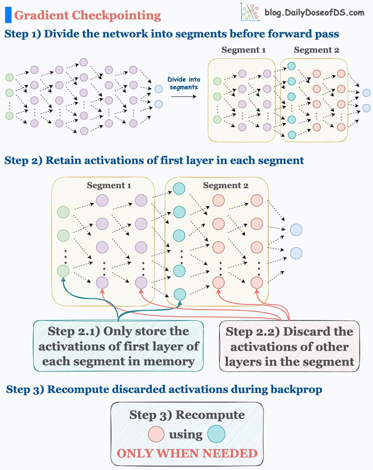
Activation checkpointing solves this problem with a simple but powerful idea: don't store all the activations; recompute them when needed.

Instead of saving the output of every layer during the forward pass, we only save the outputs at specific, pre-defined "checkpoints". Then, during the backward pass, when the autograd engine needs an intermediate activation that wasn't saved, it recomputes it by running a partial forward pass from the most recent checkpoint.

This introduces a clear trade-off:

• Memory Savings: We drastically reduce peak memory usage by not storing the bulk of the activations.
• Compute Overhead: We increase the total computation by re-running parts of the forward pass during the backward pass.

The following image provides a high-level visual of this process.

To see this trade-off in action, let's watch a short video with an excellent animation.

This visual makes the core trade-off clear. By strategically placing checkpoints, we can achieve significant memory savings at the cost of some recomputation.

3. Checkpointing Strategies: Theory vs. Practice

The crucial question for a system designer is: which activations should we checkpoint? The answer involves a fascinating intersection of theory, algorithmic complexity, and hardware reality.

The LINK article you started earlier provides an outstanding analysis of this question. We'll now dive into its core sections.

The Theoretical Optimum: Chen's O(√n) Algorithm

In a seminal 2016 paper, Tianqi Chen et al. proposed a theoretically elegant solution. It proves you can train a network with n layers using memory that scales with $O(\sqrt{n})$ instead of $O(n)$, at the cost of just one extra forward pass. Given your background in computer science, the algorithm's structure will be familiar.

The Production Strategy: Selective Checkpointing

While Chen's algorithm is asymptotically optimal, it makes a key assumption: all layers have a uniform recomputation cost. In modern Transformers, this is false. Recomputing an attention block is far more expensive than recomputing a LayerNorm.

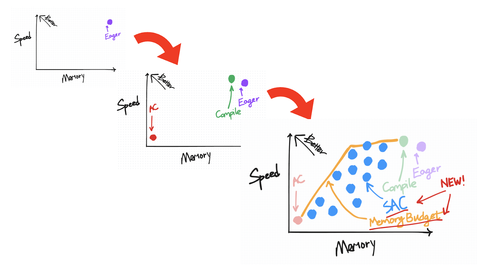
Production systems, therefore, use a more heuristic-driven selective checkpointing strategy, focusing on the trade-off between an activation's memory size and its recomputation cost.

To summarize the key findings from that reading:

• Theoretical approach (Chen's algorithm): Elegant and optimal under uniform cost assumptions. It's a foundational concept but not what's typically implemented verbatim.
• Practical approach (Selective checkpointing): More nuanced. It intelligently decides what to checkpoint based on a cost-benefit analysis: memory_saved / recomputation_cost. This is why frameworks like Megatron-LM and DeepSpeed checkpoint the outputs of entire Transformer blocks (which are computationally expensive and produce large activations) but not the individual, cheaper operations within them like LayerNorm.
• Hardware Influence: The optimal strategy is dictated by the hardware's characteristics. On modern GPUs with high compute power (Tensor Cores) but limited memory bandwidth, many operations are bandwidth-bound. Recomputing them still requires reading data from memory, making the recomputation overhead more significant than a simple FLOP count would suggest.

4. Practical Considerations and Downsides

While activation checkpointing is a vital tool, it is not a free lunch. As a systems architect, you must be aware of its potential downsides. The article LINK touches on these in its final sections, which I will summarize for you.

• Numerical Stability: Recomputing activations can introduce tiny floating-point errors because (a + b) + c is not always exactly equal to a + (b + c) in floating-point math. For sensitive models, this accumulated numerical noise can sometimes impact convergence. This is the "devil's bargain" the author refers to.
• When Not to Use It: Checkpointing is not always the right choice.
  • If you are not memory-bound, it only adds computational overhead.
  • It's for training only; it has no use in inference.
  • If your training is already bottlenecked by data loading or another factor (i.e., GPU utilization is low), adding more computation will only slow things down further.
• Implementation: In practice, this is implemented easily using library functions like torch.utils.checkpoint.checkpoint in PyTorch, which you wrap around the modules or functions you wish to checkpoint.

For a final concise summary, let's look at a brief overview from a set of lecture notes.

Conclusion

In this lesson, we have dissected activation checkpointing, a critical technique for managing memory in large-scale model training. You've gone from the fundamental concept to the deep architectural reasoning that dictates its practical application.

Key Takeaways:

• Activation checkpointing is a memory optimization technique that reduces the memory footprint of activations by trading GPU memory for additional GPU computation.
• It works by storing activations only at designated "checkpoints" and recomputing the intermediate activations during the backward pass.
• The optimal checkpointing strategy is not purely algorithmic but is heavily influenced by the underlying hardware. On modern GPUs, the trade-off must account for both recomputation cost (FLOPs) and memory bandwidth cost.
• In practice, systems use selective checkpointing, targeting computationally expensive modules (like attention and MLP blocks) while skipping cheap ones (like norms and element-wise ops).
• While powerful, the technique has a computational overhead and can introduce numerical precision issues that may affect training stability in sensitive models.

Preview of the Next Lesson:

We have now covered the main techniques for optimizing memory within a single training process: model state sharding (ZeRO/FSDP) and activation checkpointing. In the next module, we will zoom out to the datacenter level. Our next lesson will describe the overall architecture of a large-scale ML training cluster, examining how the compute, storage, and networking tiers are designed and interconnected to support the massive distributed workloads we've been discussing.