Regular Conditional Distributions: Definition and Interpretation

Recommended resources

The freely available resources this lesson will direct you to.

Hello! In our previous lesson, we successfully connected the abstract Radon-Nikodym derivative to the concrete world of econometrics. By identifying the correct measures, we rigorously derived the formula for the conditional density $f (y ∣ x)$ in a bivariate normal model and used it to recover the familiar linear expression for conditional expectation, $E [Y ∣ X = x]$ .

This lesson adds the final, crucial piece of formal machinery to our argument. So far, we have established that for any specific event $C$ in the space of $Y$ , we can define a conditional probability $P (Y \in C ∣ X = x)$ . But what allows us to speak of "the distribution of Y given X=x" as a whole? We will see that this requires one more concept: the regular conditional distribution. This is the formal object that guarantees we can coherently "stitch together" the conditional probabilities of all possible events into a valid probability distribution for each value of $x$ .

The Problem of Stitching Together Probabilities

In our previous steps, we found that for any given event $C$ , the conditional probability $P (Y \in C ∣ σ (X))$ is a random variable that is unique only up to a set of measure zero. This is the "almost everywhere" qualification that appears frequently in measure theory.

This presents a subtle but critical problem. The null set on which our definition might be ill-behaved can be different for every event $C$ . If we want to fix a single outcome $ω$ (which corresponds to a specific value $x$ for the conditioning variable $X$ ) and ask about the probability of all possible events, we would need to consider an uncountable number of such events. The union of uncountably many null sets is not necessarily a null set; it could be the entire space.

Consequently, for a given $x$ , there is no a priori guarantee that the function which maps an event $C$ to the value $P (Y \in C ∣ X = x)$ will satisfy the axioms of a probability measure (e.g., countable additivity). The following reading explains this problem concisely.

Chapter 10: Conditional probability and expectation

This excerpt from Shaw's Probability and Measure Theory directly addresses the challenge of ensuring that our collection of conditional probabilities forms a valid distribution function.

Please read the first two paragraphs of Section 10.3, starting from the introduction. The author highlights that an arbitrary version of the conditional probability P(Y \le y | \mathcal{A}) is not guaranteed to be a valid distribution function in y for a fixed outcome \omega. The simple example provided, where a valid version is modified at a single point, makes the issue very clear.

This is the core of the issue: our definition of conditional probability gives us the individual components, but we need an extra condition to ensure they assemble into a coherent whole.

Defining Regularity

The solution to this problem is to seek a "regular" version of the conditional probability. A regular conditional distribution is a special function that simultaneously satisfies two crucial properties: for each possible event, it's a valid version of the conditional probability, and for each outcome of the conditioning variable, it defines a proper probability measure.

This is formally captured in the definition of a probability kernel (also known as a Markov kernel) which serves as the regular conditional distribution.

Knowledge is the Only Good - Conditional Probability

This blog post on conditional probability provides a clear, formal definition of what makes a conditional probability "regular".

Please read the definition of a regular conditional probability (rcp) in Section 0.4. Note the three key items in the definition. In our context, \mathcal{G} is \sigma(X), and the outcome \omega corresponds to a specific value x of the conditioning variable. A function P(A, x) is a regular conditional probability of Y given X if: For a fixed event A, the function x \mapsto P(A, x) is a version of the conditional probability P(Y \in A | \sigma(X)). For a fixed value x, the function A \mapsto P(A, x) is a probability measure on the space of Y. The function x \mapsto P(A, x) is measurable. This object, P(A, x), is the rigorous answer to the question "what is the distribution of Y given X=x?"

This definition ensures that for almost every $x$ , we have a well-behaved probability measure that we can use to calculate probabilities and expectations for the variable $Y$ .

The joint density is the purple surface. For a fixed `x`, the slice through the joint density (blue curve) is not a probability density. The regular conditional density (red curve) is the normalized slice, which integrates to 1 and represents a valid probability distribution for `Y` given `X=x`.

The Existence Guarantee

Does such a "regular" object always exist? Not in general. Pathological measure spaces can be constructed where it is impossible to find a regular conditional probability. However, and this is the crucial insight for nearly all of applied statistics and econometrics, their existence is guaranteed when our random variables take values in "nice" spaces.

Technically, these are called Borel spaces. For our purposes, the most important fact is that $R^{n}$ for any $n$ is a Borel space. Since most models in finance, economics, and science map outcomes to the real numbers, this condition is almost always met.

The following theorem formalizes this existence guarantee.

Chapter 10: Conditional probability and expectation

This section states the theorem guaranteeing the existence of a regular conditional distribution function and provides an intuitive sketch of the proof.

Please read Theorem 10.15 and the proof sketch that follows, up to the end of the section (the end of the section). The key idea in the proof is to leverage the fact that the real line \mathbb{R} has a countable dense subset—the rational numbers \mathbb{Q}. The construction proceeds by: Defining the conditional distribution function F(r, \omega) for all rational numbers r. Because the rationals are countable, the set of \omega where properties like monotonicity fail is a countable union of null sets, which is itself a null set. We can therefore "repair" the function on this null set. The function is then extended from the rationals to all real numbers by right-continuity. This clever construction circumvents the problem of dealing with uncountably many null sets and is possible precisely because of the structure of the real numbers.

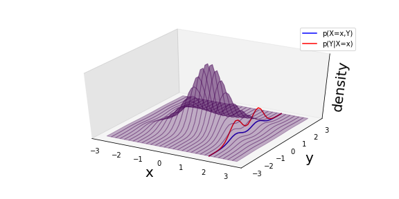
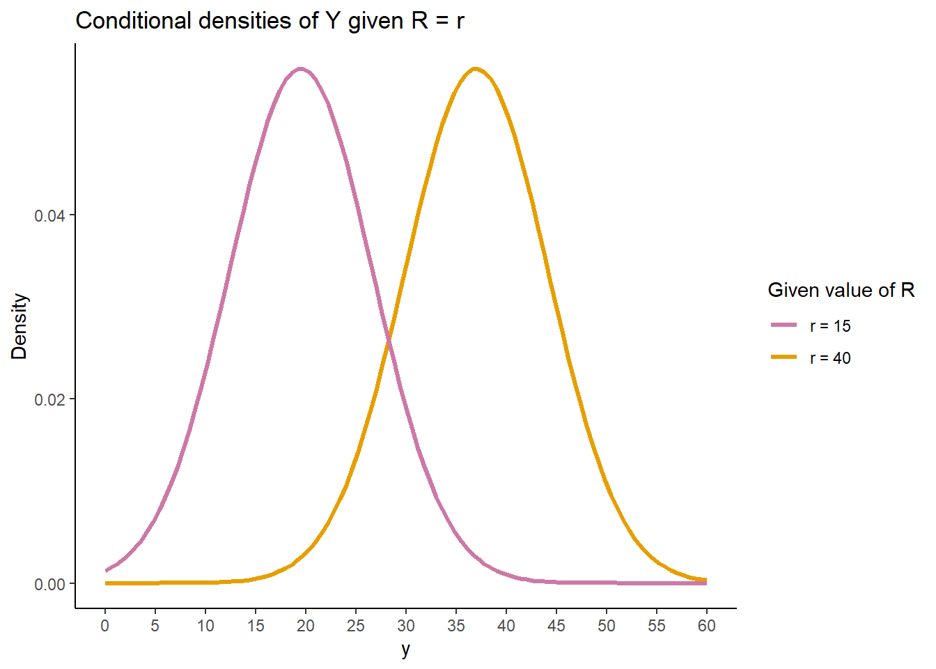
This existence theorem is the theoretical bedrock that allows us to confidently work with conditional densities like $f (y ∣ x)$ . When we derived $f (y ∣ x) = \frac{f ( x , y )}{f _{X} ( x )}$ for the bivariate normal case in the last lesson, we were finding the density of a regular conditional distribution. The theorem we've just seen provides the formal assurance that such a well-behaved family of densities exists.

This graph shows two conditional densities, one for `r=15` and one for `r=40`. The existence of a regular conditional distribution guarantees that we can find such a valid probability density for (almost) every given value of the conditioning variable `r`.

Conclusion

This lesson has introduced the final formal concept needed to complete your essay's central argument. We have moved from the conditional probability of a single event to the full conditional distribution.

Key Takeaways:

Defining conditional probability $P (Y \in C ∣ X = x)$ for each event $C$ individually is insufficient, as the "almost everywhere" property for each definition prevents us from assuming the result is a valid probability measure in $C$ for a fixed $x$ .
A regular conditional distribution is a function $P (A, x)$ that solves this by being both a version of the conditional probability for each event $A$ and a proper probability measure for each outcome $x$ .
The existence of regular conditional distributions is not universal, but a fundamental theorem guarantees their existence when random variables take values in nice spaces like $R^{n}$ (Borel spaces).
This theorem is the formal justification for the existence of well-behaved families of conditional densities, such as the $f (y ∣ x)$ we use in practical statistical modeling.

We have now assembled all the necessary theoretical components. The final step is to put them together. In our next and final lesson, we will synthesize the complete logical chain for your essay, tracing the path from the initial paradox of conditioning on a zero-probability event to its elegant resolution through the measure-theoretic framework we have built over this course.