Deriving Conditional Distributions in Bivariate Normal Models

In the last two lessons, we established the complete theoretical foundation for resolving the paradox of conditioning on zero-probability events. We first defined conditional expectation with respect to a $\sigma$-algebra, $E[Y|\mathcal{G}]$, as the formal object that captures this concept. Then, we saw that the Radon-Nikodym theorem provides the explicit mechanism for constructing this object as a specific kind of generalized density, $d\nu /dP$.

Now, we will take a step back from the abstract measure theory and ground our discussion in a concrete example from econometrics and finance. Your goal is to see how this powerful machinery connects to the practical calculations you've performed in the past. In this lesson, we will focus on a familiar model—the bivariate normal distribution—to represent the relationship between a stock's return and a market index's return. We will derive the conditional distribution using the standard "elementary" formula from your statistics courses. This will set the stage for our next lesson, where we will demonstrate how the Radon-Nikodym framework rigorously justifies this very calculation.

The Financial Context: Modeling Asset Returns

A common task in quantitative finance is to model the relationship between the return of an individual asset and the return of a broader market index. Let's define two random variables:

• $X$: The daily return of a market index (e.g., the S&P 500).
• $Y$: The daily return of a specific stock (e.g., Apple Inc.).

A standard and convenient modeling choice is to assume that the pair $(X,Y)$ follows a bivariate normal distribution. This captures the idea that both returns are individually normally distributed and that there is a linear correlation between them.

The joint probability density function (PDF) for $(X,Y)$ is given by a five-parameter function, $f(x,y)$, which depends on:

• The mean returns, ${\mu }_X$ and ${\mu }_Y$.
• The standard deviations of the returns (volatilities), ${\sigma }_X$ and ${\sigma }_Y$.
• The correlation coefficient between the returns, $\rho$.

This function describes a bell-shaped surface in three dimensions.

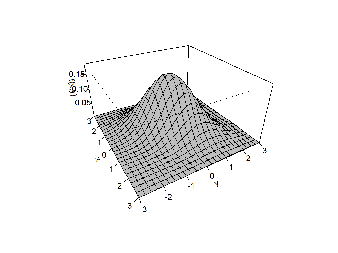
The correlation, $\rho$, determines the shape and orientation of this surface. A strong positive correlation, for example, means that when the index return $X$ is high, the stock return $Y$ is also likely to be high. A scatter plot of observations from such a distribution would show points clustered along a line with a positive slope.

Conditional Distributions: The Elementary Formula

Our central question is: "What is the distribution of the stock's return $Y$, given that the market index return $X$ was exactly some value $x$?" For instance, what is the expected return of Apple stock on a day when the S&P 500 was up exactly 1.5%?

This is a question about the conditional distribution of $Y$ given $X=x$. In your introductory econometrics and statistics courses, you learned a standard formula for the conditional PDF in the continuous case.

The following textbook chapter provides the formal definitions for joint, marginal, and conditional distributions for continuous random variables.

As you just read, the conditional density of $Y$ given $X=x$ is defined as:

$$f(y|x)=\frac{f(x,y)}{f_X(x)}$$

where $f(x,y)$ is the joint PDF and $f_X(x)$ is the marginal PDF of $X$.

At this point, the core of our essay's argument should be clear. Since $X$ is a continuous random variable, the probability of the event $\{X=x\}$ is zero. The formula above appears to be a division of zero by zero, as both $f(x,y)dxdy$ and $f_X(x)dx$ approach zero. This is precisely the paradox that necessitates a more rigorous, measure-theoretic approach.

Intuitively, however, we can think of this process as taking a "slice" through the 3D joint probability surface at a specific value of $X$. The shape of this slice, once rescaled so that its area is 1, gives us the conditional probability distribution.

The following video provides an excellent visual and intuitive explanation of this "slicing" concept.

Deriving the Conditional Distribution for the Bivariate Normal

Let's now apply the formula $f(y|x)=f(x,y)/f_X(x)$ to our bivariate normal model. The goal is to find the exact form of the conditional distribution of $Y$ given $X=x$. It is a known result that this conditional distribution is also normal. Our task is to find its mean and variance.

The derivation involves substituting the complex formulas for the bivariate normal joint PDF and the univariate normal marginal PDF, followed by some algebraic simplification. The video below provides a clear, step-by-step walkthrough of this derivation.

As you saw in the video, the algebraic manipulation reveals two key results. For the bivariate normal model $(X,Y)$, the conditional distribution of $Y$ given $X=x$ is a normal distribution with:

1. Conditional Mean:

   $$E[Y|X=x]={\mu }_Y+\rho \frac{{\sigma }_Y}{{\sigma }_X}(x-{\mu }_X)$$

2. Conditional Variance:

   $$\text{Var}(Y|X=x)={\sigma }_Y^2(1-{\rho }^2)$$

For completeness, the full algebraic derivation, which involves completing the square in the exponent of the exponential function, is laid out in the following resource.

Notice the structure of these results. The conditional mean is a linear function of $x$. This is, in fact, the population regression line of $Y$ on $X$. The conditional variance is a constant that does not depend on $x$. This property is known as homoscedasticity, a familiar concept from your econometrics background.

Conclusion

In this lesson, we stepped away from abstract measure theory to perform a concrete calculation rooted in financial econometrics. We used the familiar, if seemingly paradoxical, formula for conditional density to analyze the bivariate normal distribution.

Key Takeaways:

• For two variables $(X,Y)$ following a bivariate normal distribution, the conditional distribution of $Y$ given $X=x$ is also a normal distribution.
• The conditional mean, $E[Y|X=x]$, is a linear function of $x$, corresponding to the linear regression of $Y$ on $X$.
• The conditional variance, $\text{Var}(Y|X=x)$, is constant and equals ${\sigma }_Y^2(1-{\rho }^2)$.
• We derived this result using the elementary formula $f(y|x)=f(x,y)/f_X(x)$, temporarily setting aside the "division by zero" paradox.

We have now established a concrete result using standard methods. The final piece of your essay's argument is to show how the rigorous Radon-Nikodym framework justifies this calculation. In our next lesson, we will do exactly that. We will identify the specific measures $\nu$ and $P$ for this bivariate normal case, verify absolute continuity, and show that the resulting Radon-Nikodym derivative produces the very same conditional density we found here. This will connect the abstract theory to practical application, completing the core argument.