Radon-Nikodym Derivative and Conditional Expectation in Bivariate Normal Distributions

Recommended resources

The freely available resources this lesson will direct you to.

[PDF] E. Vitali Lecture 5. Conditional Expectation So far we have focussed ...phd.fisica.unimi.it
[PDF] Continuous Random Variables II - MIT OpenCourseWareocw.mit.edu

Welcome back. In our last lesson, we took a crucial step in formalizing our bivariate normal model of asset returns. We translated the joint and marginal densities into their corresponding measures, $ν$ and $P_{X}$ , and verified that $ν$ is absolutely continuous with respect to $P_{X}$ . This verification was the key that unlocked the use of the Radon-Nikodym theorem, guaranteeing the existence of a derivative $\frac{d ν}{d P _{X}}$ which serves as the rigorous definition of conditional probability.

In this lesson, we will move from existence to construction. We will explicitly compute this Radon-Nikodym derivative and demonstrate that it precisely recovers the familiar formula for conditional probability you've used in your econometrics work. We will then use this to calculate the conditional expectation $E [Y ∣ X = x]$ for the bivariate normal case and show that it yields the exact linear relationship you encountered in your previous studies, thereby closing the loop between abstract measure theory and practical statistical modeling.

From the Abstract Derivative to a Concrete Formula

Let's begin by recalling the setup from the previous lesson. We have two measures on the space of the conditioning variable $X$ , which is $(R, B (R))$ . For a fixed event of interest $C$ in the space of $Y$ (e.g., $Y \leq y_{0}$ ), these measures are:

$ν (B) = P (X \in B, Y \in C) = \int_{B} (\int_{C} f (x, y) d y) d x$
$P_{X} (B) = P (X \in B) = \int_{B} f_{X} (x) d x$

The Radon-Nikodym theorem guarantees the existence of a $σ (X)$ -measurable function, which we can write as $g (X)$ , that is the derivative of $ν$ with respect to $P_{X}$ . This function is defined by the property:

ν (B) = \int_{B} g (x) d P_{X} (x) for any Borel set B \subseteq R

Our task is to find the function $g (x)$ .

We know that the measure $P_{X}$ has a density $f_{X} (x)$ with respect to the Lebesgue measure $λ$ . This means we can write $d P_{X} (x) = f_{X} (x) d x$ . Substituting this and our definition of $ν (B)$ into the defining equation gives:

\int_{B} (\int_{C} f (x, y) d y) d x = \int_{B} g (x) f_{X} (x) d x

This equation must hold for every possible choice of the set $B$ . The only way for this to be true is if the integrands on both sides are equal (almost everywhere with respect to Lebesgue measure). Therefore, we must have:

\int_{C} f (x, y) d y = g (x) f_{X} (x)

Solving for our Radon-Nikodym derivative $g (x)$ gives us an explicit formula:

g (x) = \frac{\int _{C} f ( x , y ) d y}{f _{X} ( x )}

This function $g (x)$ is the rigorous, measure-theoretic definition of the conditional probability $P (Y \in C ∣ X = x)$ . Notice that if we take the derivative of this expression with respect to $y$ (assuming $C = (- \infty, y]$ to get a CDF), we intuitively arrive at the conditional probability density function:

f (y ∣ x) = \frac{f ( x , y )}{f _{X} ( x )}

This is a remarkable result. It demonstrates that the abstract machinery of the Radon-Nikodym theorem leads directly to the elementary formula for conditional density that you're familiar with from your statistics and econometrics courses. The formula isn't just a convenient heuristic; it's a direct consequence of the rigorous definition of conditional probability.

Explicit Calculation of Conditional Expectation

Now let's apply this to compute the conditional expectation, $E [Y ∣ X]$ . This is defined as a $σ (X)$ -measurable random variable, let's call it $h (X)$ , that satisfies certain properties. The most direct way to compute its value $h (x) = E [Y ∣ X = x]$ is to take the expectation of $Y$ with respect to the conditional distribution we just found.

h (x) = E [Y ∣ X = x] = \int_{- \infty}^{\infty} y \cdot f (y ∣ x) d y = \int_{- \infty}^{\infty} y \frac{f ( x , y )}{f _{X} ( x )} d y

The following reading walks through this exact logic and applies it to our case of interest: the bivariate normal distribution.

[PDF] E. Vitali Lecture 5. Conditional Expectation So far we have focussed ...

This section from Vitali's lecture notes provides the crucial bridge from the abstract definition to a practical calculation. It demonstrates how, under the assumption of a joint density, the conditional expectation E[X|Y] can be computed as a function g(Y), and then carries out this computation for the bivariate normal case.

Please read section IV. AN EXPLICIT CALCULATION. Pay close attention to the derivation that starts from the definition of conditional density and arrives at the conclusion that E[X|Y] = g(Y), where g(y) = \int dx \, x \, p(x|y). Then, follow the example for a bivariate normal. The author computes E[X|Y=y]. In our problem, we are interested in E[Y|X=x], so you will just need to mentally swap the roles of X and Y. The final formula shows that the conditional expectation is a linear function of the conditioning variable.

As the reading demonstrates, for a bivariate normal random variable $(X, Y)$ with means $(μ_{X}, μ_{Y})$ , variances $(σ_{X}^{2}, σ_{Y}^{2})$ , and correlation $ρ$ , the conditional expectation of $Y$ given $X = x$ is:

E [Y ∣ X = x] = μ_{Y} + ρ \frac{σ _{Y}}{σ _{X}} (x - μ_{X})

This is the celebrated result from linear regression and econometrics. We have now shown that this formula is not merely the best linear predictor, but, in the specific case of joint normality, it is the true conditional expectation, derived rigorously through the Radon-Nikodym framework. You have now connected the abstract definition $E [Y ∣ σ (X)]$ to the concrete formula you would use to predict an asset's return given a specific market index value.

Visualizing the Result

These abstract calculations have a very clear and intuitive visual interpretation.

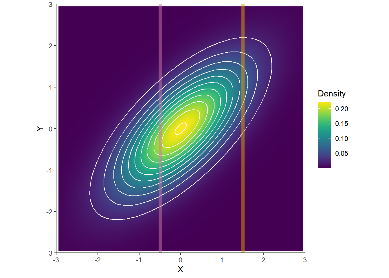
A contour and heatmap plot of a bivariate normal joint probability density function, $f(x,y)$. The vertical lines represent taking a 'slice' of the distribution at fixed values of X, for example at X = -0.5 and X = 1.5.

The image above shows the joint density of $(X, Y)$ . The process of conditioning on $X = x$ is like taking a vertical slice through this two-dimensional distribution. The profile of the density along that slice gives you the shape of the conditional distribution of $Y$ .

The resulting conditional probability density functions, $f(y|x)$, for the two slices taken at X = -0.5 (pink) and X = 1.5 (orange). Both are normal distributions, but with different means.

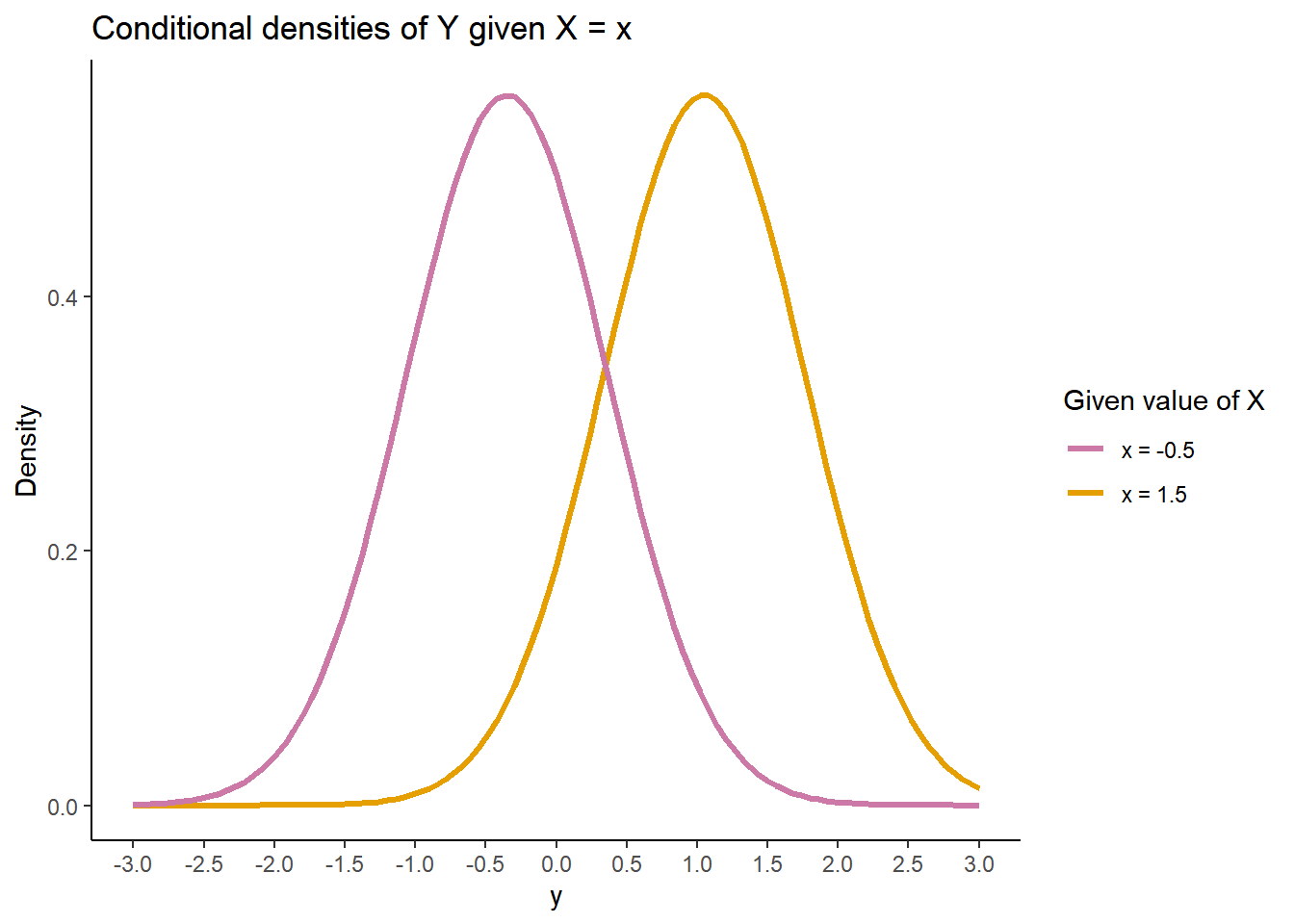
The second image shows the normalized results of taking those slices. Each slice, when normalized to integrate to 1, is a valid probability density function. For the bivariate normal case, these conditional distributions are themselves normal. The key insight from our calculation is that the mean of these conditional distributions shifts as we change the value of $x$ we are conditioning on. Our derived formula, $E [Y ∣ X = x] = μ_{Y} + ρ \frac{σ _{Y}}{σ _{X}} (x - μ_{X})$ , tells us exactly how the center of this bell curve moves: it moves linearly with $x$ . The mean of the orange curve (conditional on $X = 1.5$ ) is higher than the mean of the pink curve (conditional on $X = - 0.5$ ), just as the formula predicts for a positive correlation $ρ$ .

Conclusion

In this lesson, we have successfully closed the loop on the main part of your essay's argument. We have demonstrated how the abstract machinery of measure theory provides a solid foundation for the practical calculations of conditional probability and expectation.

Key Takeaways:

The Radon-Nikodym derivative, which provides the formal definition of conditional probability, can be explicitly calculated.
This calculation shows that the derivative corresponds directly to the familiar ratio of densities: $P (Y \in C ∣ X = x) = \frac{\int _{C} f ( x , y ) d y}{f _{X} ( x )}$ . This justifies the use of the elementary formula $f (y ∣ x) = f (x, y) / f_{X} (x)$ for conditional densities.
Applying this to compute the conditional expectation for a bivariate normal distribution rigorously reproduces the well-known linear formula $E [Y ∣ X = x] = μ_{Y} + ρ \frac{σ _{Y}}{σ _{X}} (x - μ_{X})$ .
This proves that the standard formula used in econometrics is not just an ad-hoc tool but is the correct and unique conditional expectation under the measure-theoretic framework.

We have almost completed our argument. There is one final piece of formal machinery to address: what guarantees that we can always find such a nice, well-behaved family of conditional distributions $f (y ∣ x)$ for every $x$ ? In our next lesson, we will introduce the concept of a regular conditional distribution, which is the formal object that provides this guarantee and puts the final polish on our rigorous understanding.