Building Pro Formas: Python for NPV and IRR

Hello! Welcome back to your course on real estate investment metrics.

In our last few lessons, we've focused on the core concepts of the time value of money, calculating Net Present Value (NPV) to determine an investment's value in today's euros, and Internal Rate of Return (IRR) to find its projected annualized return. These are powerful, but they rely on a crucial input: a series of projected cash flows.

Today, we will tie everything together. Your learning outcome is to write Python code to build a multi-year pro forma and calculate NPV and IRR. A pro forma is a forward-looking financial statement that projects an investment's performance over a holding period. It is the engine that generates the cash flow projections we need for our NPV and IRR calculations. Building this model in Python will give you a dynamic and reusable tool for analyzing any potential deal.

1. The Anatomy of a Pro Forma

Before we start coding, let's understand what we're building. A multi-year pro forma is essentially a story about the investment, told in numbers. It starts with the purchase and projects all the income, expenses, and financing costs over the time you plan to own the property, and ends with the projected sale.

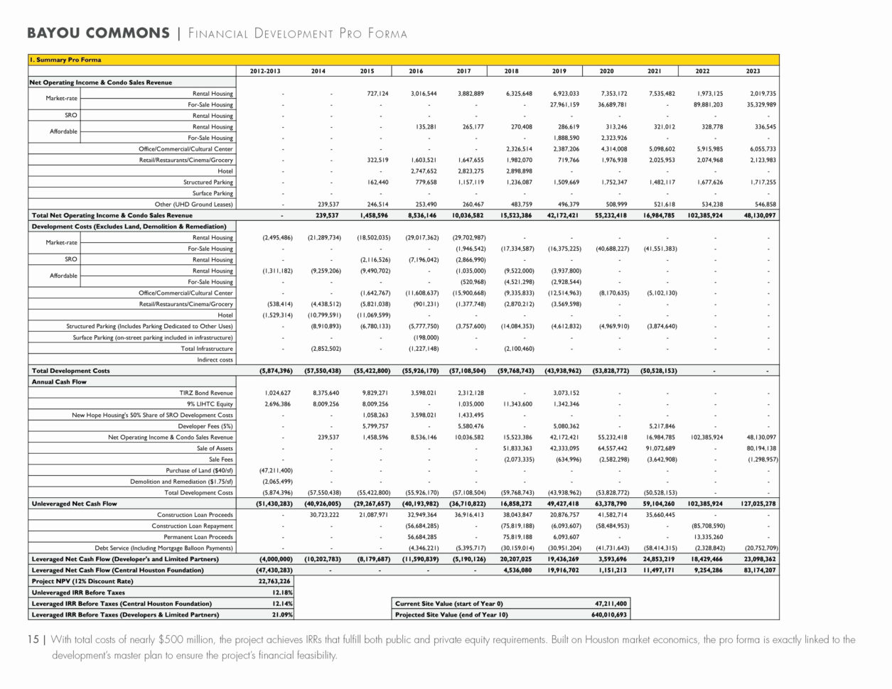
Look at the image below. It's a complex pro forma for a large development project, but it contains all the core elements we'll be modeling today: revenue projections, cost projections, the resulting annual cash flows, and key summary metrics like NPV and IRR.

To build our own version, we need to gather a set of assumptions. To get a clear idea of what these are, please read the introductory section of the following article.

As you can see, our model will need to account for everything from the down payment and mortgage details to the costs of selling the property years down the line.

2. Building the Pro Forma in Python, Step-by-Step

Now, let's translate these components into code. Our goal is to create a function that takes these inputs and returns the NPV and IRR. We will use the numpy_financial library, which you've used in previous lessons.

To see the npv and irr functions in action again as a quick refresher, you can review this video.

Our Python model will perform the following logical steps:

1. Initialize inputs: Define all our assumptions as variables.
2. Project annual operations: Loop through the holding period to calculate Gross Rent, Vacancy, Operating Expenses, and finally, Net Operating Income (NOI) for each year, applying growth assumptions.
3. Factor in financing: Calculate the annual mortgage payment (debt service) and subtract it from NOI to find the Pre-Tax Cash Flow for each year.
4. Model the exit: Calculate the projected sale price (Reversion Value) at the end of the holding period and subtract selling costs and the remaining loan balance to find the Net Sale Proceeds.
5. Assemble the final cash flow series: Create a single list containing:
   • The initial investment (a negative number).
   • The annual Pre-Tax Cash Flows for the holding period.
   • The final year's cash flow, which includes the Net Sale Proceeds.
6. Calculate final metrics: Run the npf.npv and npf.irr functions on this final cash flow series.

The article from Shane Chang provides a complete Python function that implements exactly this logic.

An Alternative Approach: Using pandas

For someone with your software engineering background, it's worth noting that financial models like this are often built using the pandas library. pandas DataFrames and Series can make handling time-series data even more intuitive.

The article below demonstrates how to build a similar DCF model using pandas. You don't need to implement this now, but it's a valuable perspective on how to structure financial data for more complex analysis, such as the Monte Carlo simulations we'll cover later in the course.

3. Putting it all Together: A Practical Example

Let's consolidate the code from the shanechang.com article into a single, runnable script. Here is the complete model. I've added comments to clarify each step, linking back to the concepts we've learned.

import numpy as np
import numpy_financial as npf

def calculate_real_estate_investment(
    purchase_price,
    down_payment_percent,
    mortgage_interest_rate,
    loan_term_years,
    monthly_rent,
    property_tax_rate,
    insurance_rate,
    maintenance_rate,
    management_fee_rate,
    vacancy_rate,
    appreciation_rate,
    expense_growth_rate,
    rent_growth_rate,
    sales_commission_rate,
    holding_period_years,
    discount_rate
):
    """
    Builds a multi-year pro forma for a rental property and calculates NPV and IRR.
    """
    # --- 1. Initial Investment ---
    down_payment = purchase_price * down_payment_percent
    loan_amount = purchase_price - down_payment
    initial_investment = down_payment # In a real scenario, this would include closing costs.

    # --- 2. Annual Projections (Pro Forma) ---
    annual_cash_flows = []
    current_property_value = purchase_price
    current_monthly_rent = monthly_rent
    
    # Calculate fixed monthly mortgage payment
    monthly_mortgage = -npf.pmt(mortgage_interest_rate / 12, loan_term_years * 12, loan_amount)
    annual_debt_service = monthly_mortgage * 12

    # Store mortgage balance over time
    mortgage_balances = []
    remaining_balance = loan_amount

    for year in range(1, holding_period_years + 1):
        # --- Project Income ---
        gross_potential_rent = current_monthly_rent * 12
        vacancy_loss = gross_potential_rent * vacancy_rate
        effective_gross_income = gross_potential_rent - vacancy_loss

        # --- Project Operating Expenses ---
        property_taxes = current_property_value * property_tax_rate
        insurance = current_property_value * insurance_rate
        maintenance = current_property_value * maintenance_rate
        management_fees = effective_gross_income * management_fee_rate
        total_op_expenses = property_taxes + insurance + maintenance + management_fees

        # --- Calculate NOI and Pre-Tax Cash Flow ---
        noi = effective_gross_income - total_op_expenses
        pre_tax_cash_flow = noi - annual_debt_service
        annual_cash_flows.append(pre_tax_cash_flow)
        
        # --- Update values for next year ---
        current_property_value *= (1 + appreciation_rate)
        current_monthly_rent *= (1 + rent_growth_rate)
        
        # Update remaining mortgage balance (simplified for this model)
        # A full amortization schedule would be more precise
        principal_paid = 0
        temp_balance = remaining_balance
        for _ in range(12):
            interest_payment = temp_balance * (mortgage_interest_rate / 12)
            principal_payment = monthly_mortgage - interest_payment
            principal_paid += principal_payment
            temp_balance -= principal_payment
        remaining_balance -= principal_paid
        mortgage_balances.append(remaining_balance)


    # --- 3. Exit (Reversion) Calculation ---
    projected_sale_price = current_property_value
    sales_commission = projected_sale_price * sales_commission_rate
    remaining_mortgage = mortgage_balances[-1] if mortgage_balances else loan_amount
    net_sale_proceeds = projected_sale_price - sales_commission - remaining_mortgage
    
    # Add net sale proceeds to the last year's cash flow
    annual_cash_flows[-1] += net_sale_proceeds

    # --- 4. Final Cash Flow Series for NPV/IRR ---
    # Combine initial investment with all future cash flows
    full_cash_flow_series = [-initial_investment] + annual_cash_flows

    # --- 5. Calculate Metrics ---
    net_present_value = npf.npv(discount_rate, full_cash_flow_series)
    internal_rate_of_return = npf.irr(full_cash_flow_series)

    return {
        "npv": net_present_value,
        "irr": internal_rate_of_return,
        "annual_cash_flows": annual_cash_flows,
        "net_sale_proceeds": net_sale_proceeds
    }

# --- Example Usage ---
if __name__ == '__main__':
    property_inputs = {
        "purchase_price": 500000,
        "down_payment_percent": 0.20,
        "mortgage_interest_rate": 0.035, # Assuming Spanish market rates
        "loan_term_years": 30,
        "monthly_rent": 2000,
        "property_tax_rate": 0.008, # Based on Spanish IBI (Impuesto sobre Bienes Inmuebles)
        "insurance_rate": 0.003,
        "maintenance_rate": 0.01,
        "management_fee_rate": 0.08,
        "vacancy_rate": 0.05,
        "appreciation_rate": 0.02,
        "expense_growth_rate": 0.02, # Not used in this simplified model, but good to have
        "rent_growth_rate": 0.02,
        "sales_commission_rate": 0.05, # Typical Spanish agency fees
        "holding_period_years": 10,
        "discount_rate": 0.08 # Your required rate of return
    }

    results = calculate_real_estate_investment(**property_inputs)

    print(f"Investment Analysis:")
    print(f"  Net Present Value (NPV): {results['npv']:,.2f} €")
    print(f"  Internal Rate of Return (IRR): {results['irr']:.2%}")
    print("\nProjected Annual Pre-Tax Cash Flows:")
    for i, cf in enumerate(results['annual_cash_flows']):
        if i < len(results['annual_cash_flows']) - 1:
            print(f"  Year {i+1}: {cf:,.2f} €")
        else:
            # Last year includes sale proceeds
            print(f"  Year {i+1} (incl. sale): {cf:,.2f} €")

Conclusion

Congratulations! You have now built a complete, multi-year financial model in Python. This is a significant milestone that combines concepts from all previous lessons into a single, powerful analytical tool. This script forms the foundation upon which all further analysis—including Spanish taxes, different ownership structures, and risk modeling—will be built.

Key Takeaways:

• A pro forma is a financial projection of an investment's future performance over a holding period.
• It integrates income, operating expenses, financing, and exit assumptions to generate a series of net cash flows.
• Using Python and numpy_financial, you can automate the creation of the pro forma and the calculation of NPV and IRR.
• This model allows for rapid "what-if" analysis by changing input variables to see their impact on profitability.

Preview of the Next Lesson:
Our pro forma relies on the "Income Approach" to valuation, using discounted cash flows. But how do we know if our purchase price and exit value assumptions are reasonable? To answer that, we need to look at the market. In our next lesson, we will begin a new module on advanced valuation by learning to describe the methodology of the Sales Comparison Approach, the primary method used by appraisers to determine a property's market value by comparing it to similar, recently sold properties.