Taylor Expansions for Multivariable Functions

Recommended resources

The freely available resources this lesson will direct you to.

Welcome to the next lesson in our journey through multivariable calculus. In our previous session, we introduced the Hessian matrix and saw how its eigenvalues reveal the local curvature of a function's surface. This gave us a powerful tool to understand the geometry at a specific point—whether it's bowl-shaped, dome-shaped, or a saddle.

Today, we will synthesize this concept with the gradient to construct one of the most fundamental tools in applied mathematics: the Taylor expansion for multivariable functions. Just as Taylor series in single-variable calculus allow us to approximate complex functions with simple polynomials, their multivariable counterparts let us approximate complex surfaces with planes and quadratic shapes. This is the theoretical bedrock for many optimization algorithms, including Newton's method, which you'll encounter in deep learning.

Our goal is to construct and understand both the first-order (linear) and second-order (quadratic) Taylor approximations.

From Tangent Lines to Tangent Planes

Let's start by recalling the Taylor expansion for a single-variable function $f (x)$ around a point $a$ :

f (x) \approx f (a) + f^{'} (a) (x - a) + \frac{1}{2 !} f^{''} (a) (x - a)^{2} + \dots

The first-order approximation, $L (x) = f (a) + f^{'} (a) (x - a)$ , gives the tangent line to the function at $a$ . It's the best linear approximation of the function near that point.

Now, consider a scalar-valued function of multiple variables, $f (x)$ , where $x \in R^{n}$ . We want to approximate this function near a point $a$ .

The first-order term in the 1D case is the product of the derivative and the displacement, $f^{'} (a) (x - a)$ . In the multivariable world, the derivative is captured by the gradient, $\nabla f (a)$ , and the displacement is the vector $(x - a)$ .

How would you combine the gradient vector $\nabla f (a)$ and the displacement vector $(x - a)$ to produce a scalar value analogous to the 1D term $f^{'} (a) (x - a)$ ?

This operation is precisely the dot product, which projects the displacement vector onto the direction of steepest ascent. This gives us the first-order Taylor expansion, also known as the linear or tangent plane approximation:

f (x) \approx f (a) + \nabla f (a) \cdot (x - a)

This equation defines a hyperplane (a plane in 3D) that is tangent to the surface of $f (x)$ at the point $a$ . It has the same value $f (a)$ and the same "slope" (gradient) at that point.

The following video provides an excellent visual intuition for how these approximations build up from a constant value (zeroth-order) to a tangent plane (first-order) and finally to a curved surface (second-order).

M4ML - Multivariate Calculus - 4.8 Multivariate Taylor

This video from Imperial College London, "M4ML - Multivariate Taylor," demonstrates how Taylor approximations look as surfaces.

Watch the segment from the visual demonstration. Pay attention to how the zeroth-order approximation is a flat plane, and the first-order approximation is a tilted plane that matches the function's gradient at the point of expansion.

Incorporating Curvature: The Second-Order Approximation

The linear approximation is good, but it's flat. It completely ignores the curvature we studied in the last lesson. To create a better approximation, we need to include a second-order term.

In the 1D case, this term is $\frac{1}{2} f^{''} (a) (x - a)^{2}$ . It involves the second derivative and the square of the displacement. For the multivariable case, the second derivative is the Hessian matrix, $H_{f} (a)$ , and the displacement is the vector $(x - a)$ .

Drawing on our previous lesson, how can we combine the Hessian matrix with two instances of the displacement vector to produce a scalar value that represents curvature's effect?

You're right, this calls for the quadratic form $v^{T} H v$ we explored previously. Here, the vector $v$ is our displacement vector $(x - a)$ . By adding this term, we arrive at the second-order Taylor expansion:

f (x) \approx f (a) + \nabla f (a) \cdot (x - a) + \frac{1}{2} (x - a)^{T} H_{f} (a) (x - a)

This is no longer a flat plane but a quadratic surface (a paraboloid or hyperboloid) that approximates the original function. It matches the function's value, its gradient, and its curvature (as defined by the Hessian) at the point $a$ .

This image visualizes the concepts we're discussing. The gray, wavy surface is the original function $f(x,y)$. The blue plane is the first-order Taylor approximation (tangent plane) at the center point. A second-order approximation would be a curved surface that "hugs" the gray surface more closely than the plane does.

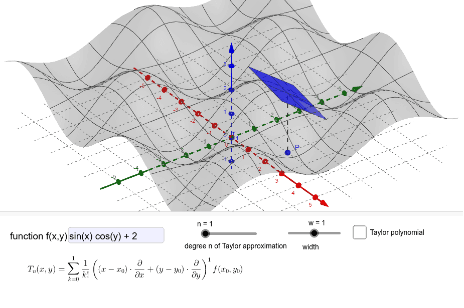
The following resource provides a clear, concise summary of these formulas and presents them in the compact matrix notation that is standard in machine learning.

Hessian Matrix, Taylor Series, and the Newton-Raphson ...

This article from PyImageSearch lays out the formulas for multivariable Taylor series in a very practical way.

Please read the sections titled "Linearization" and "Taylor Series Expansion". Focus on the equations for the first-order approximation and the second-order approximation. Notice how the gradient and Hessian slot perfectly into the general Taylor series structure.

A Concrete Example

Let's solidify this with a worked example from the same article. We'll find the first and second-order approximations for the function $f (x_{1}, x_{2}) = e^{x_{1}} + sin (x_{2})$ around the point $x_{0} = (1, 1)$ .

The process involves:

Evaluating the function at the point: $f (1, 1)$ .
Computing the gradient $\nabla f (x)$ and evaluating it at $(1, 1)$ .
Computing the Hessian $H (x)$ and evaluating it at $(1, 1)$ .
Plugging these components into the Taylor expansion formulas.

Hessian Matrix, Taylor Series, and the Newton-Raphson ...

Let's continue with the PyImageSearch article.

Read through the short example that begins just after the second figure. It shows the calculation of the gradient and Hessian for the example function and then assembles the first- and second-degree polynomial approximations.

This process demonstrates how the abstract formulas translate into a concrete computational recipe. In practice, libraries like PyTorch or JAX would compute these derivatives automatically, but understanding the underlying structure is crucial.

Taylor's Theorem: Making the Approximation Exact

So far, we've used the "approximately equal" sign ( $\approx$ ). But how good is this approximation? Taylor's Theorem provides the answer by giving an exact expression that includes a remainder term. The most intuitive form is the Lagrange remainder.

For the second-order expansion, the theorem states that there exists some point $c$ on the line segment connecting $a$ and $x$ such that:

f (x) = f (a) + \nabla f (a) \cdot (x - a) + \frac{1}{2} (x - a)^{T} H_{f} (c) (x - a)

Notice the only difference: the Hessian is evaluated at this intermediate point $c$ , not at $a$ . This means the error in our quadratic approximation is determined by how much the Hessian changes between $a$ and $x$ . If the function has very stable, slowly-changing curvature, our approximation will be excellent.

The proof of this theorem is a beautiful piece of calculus. It works by reducing the multivariable problem to a single-variable problem along the line connecting $a$ and $x$ , and then applying the familiar 1D Taylor's theorem.

To see how this is formally stated and derived, let's look at a more rigorous resource.

Taylor Series and Taylor's Theorem for Multivariable Functions, Real Analysis II

This video, "Taylor Series and Taylor's Theorem for Multivariable Functions" by Dr. Bevin Maultsby, provides a formal proof.

Watch from the statement of the theorem. The instructor carefully lays out the full theorem, including the Taylor polynomial and the Lagrange remainder term. The key insight is that the remainder term looks almost identical to the next term in the series, but the derivative is evaluated at an unknown point c on the line segment between p and x. Then, watch the setup of the proof from parameterizing the line segment, which introduces the core strategy of defining a single-variable function h(t) by evaluating f along the line.

This reduction to a 1D problem is a common and powerful technique in multivariable analysis, elegantly connecting complex higher-dimensional concepts back to the foundational principles of single-variable calculus.

Conclusion

In this lesson, we have assembled the gradient and the Hessian into the multivariable Taylor series, a tool for creating local polynomial approximations of complex functions.

Key Takeaways:

The first-order Taylor expansion approximates a function with a tangent hyperplane, using the function's value and gradient at a point.
$f (x) \approx f (a) + \nabla f (a) \cdot (x - a)$
The second-order Taylor expansion provides a more accurate quadratic approximation by also matching the function's curvature via the Hessian.
$f (x) \approx f (a) + \nabla f (a) \cdot (x - a) + \frac{1}{2} (x - a)^{T} H_{f} (a) (x - a)$
Taylor's Theorem makes these approximations exact by adding a remainder term, which depends on higher-order derivatives at an intermediate point.

You now possess the complete analytical toolkit for describing the local behavior of a multivariable function. In our next and final lesson of this module, we will apply these Taylor expansions at critical points (where $\nabla f = 0$ ) to formally derive the second derivative test and classify these points as local minima, maxima, or saddle points.