Gradients: Direction of Steepest Ascent

Recommended resources

The freely available resources this lesson will direct you to.

Introduction

In our previous lesson, we established how to measure a multivariable function's rate of change along the primary coordinate axes using partial derivatives. This gave us the slope of the function's surface if we only moved parallel to the x-axis or the y-axis. However, for optimization, this is not enough. We need to answer a more fundamental question: from any given point on a surface, which direction is the steepest way up? And, more importantly for minimizing error, which way is the steepest way down?

Today, we will assemble the partial derivatives we learned about into a single, powerful vector: the gradient. This lesson will formally define the gradient and, through the concept of the directional derivative, establish its core geometric meaning. You will learn not only how to compute the gradient but also why it represents the direction of a function's most rapid change—a foundational principle for virtually all iterative optimization algorithms in machine learning.

From Partial Derivatives to a Full Vector

In the last lesson, we took a function like $f (x, y)$ and computed its partial derivatives $\frac{\partial f}{\partial x}$ and $\frac{\partial f}{\partial y}$ separately. Each of these is a scalar function that tells us the rate of change in one specific direction. The natural next step is to combine them.

The gradient of a scalar-valued function $f : R^{n} \to R$ at a point $x$ is the vector of its partial derivatives at that point. We denote it with the symbol $\nabla$ (nabla). For a function of two variables, it's a 2D vector:

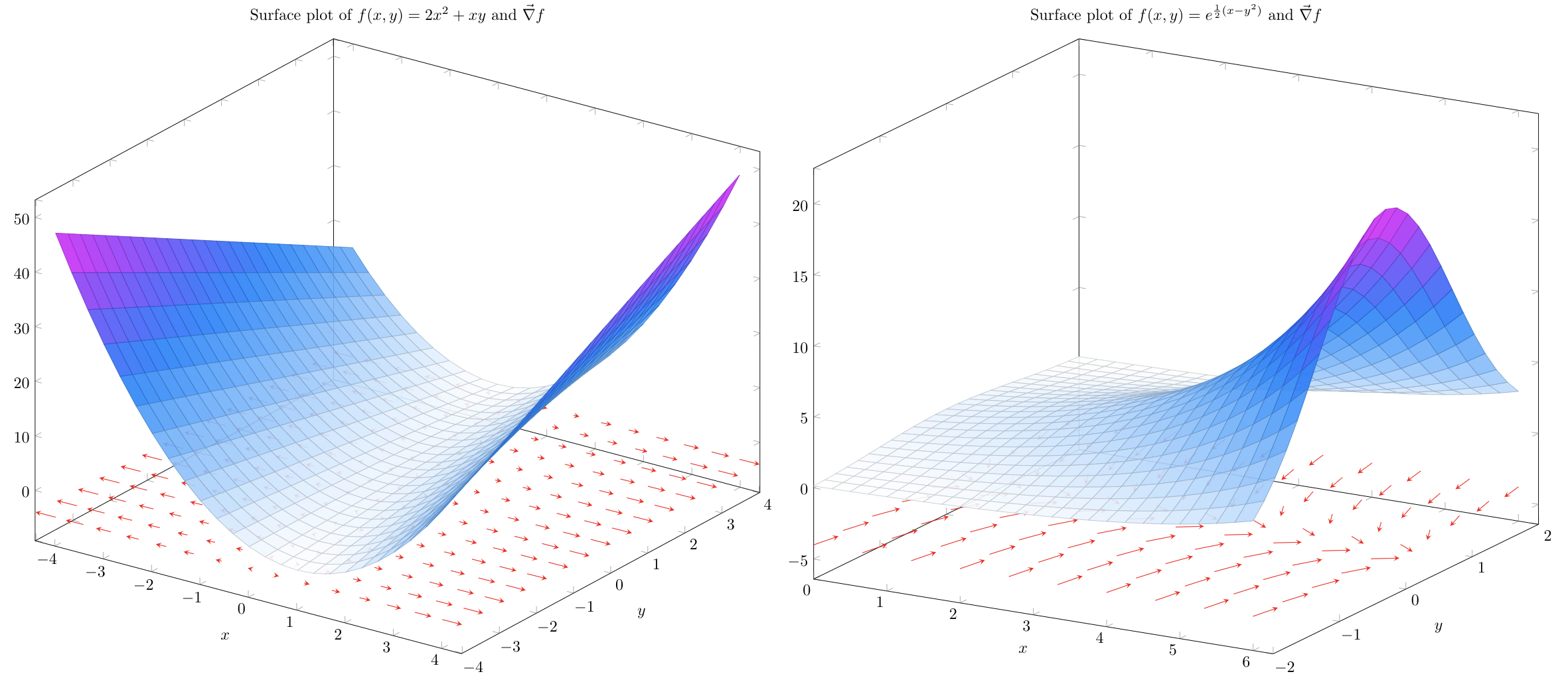
\nabla f (x, y) = [\frac{\partial f}{\partial x} (x, y) \frac{\partial f}{\partial y} (x, y)]

This vector now lives in the input space of the function. If $f$ describes a surface over the xy-plane, $\nabla f$ is a 2D vector in that plane.

The text below offers a crisp definition and a useful clarification on the different ways mathematicians and computer scientists use the term "gradient".

Appendix A: Gradients Review — Deep Learning with PyTorch

This document provides a concise review of gradients from a machine learning perspective.

Please read the sections "Ingredient 4: Gradients" and "Gradients intuition". Pay close attention to the table that distinguishes the gradient as an operator (\nabla), a function (\nabla f), and a value (a specific vector at a point). This precision is valuable in systems programming and mathematics.

As you just read, the gradient is a vector field. At every point $(x, y)$ in the domain, the gradient $\nabla f (x, y)$ gives us a vector with a specific direction and magnitude. Intuitively, these vectors point "uphill" on the function's surface.

On the left is the surface for $f(x, y) = 2x^2 + xy$ and on the right is $f(x, y) = e^{-(x-3)^2} + e^{-(y-1)^2}$. The red arrows in the plane below each surface represent the gradient vector field $\nabla f$. Notice how the arrows point towards areas where the function value is increasing, and their length (magnitude) is larger where the surface is steeper.

The Directional Derivative: Proving the Gradient's Power

The intuition that the gradient points "uphill" is powerful, but we need to prove it. To do this, we must first generalize partial derivatives to measure the rate of change in any arbitrary direction, not just along the axes. This is the role of the directional derivative.

The directional derivative of a function $f$ at a point $a$ in the direction of a unit vector $u$ is denoted $D_{u} f (a)$ . It turns out there's a beautifully simple formula connecting it to the gradient:

D_{u} f (a) = \nabla f (a) \cdot u

This formula states that the rate of change in any direction $u$ is simply the projection of the gradient vector onto that direction. This is the key to understanding the gradient's properties.

Let's watch a video that derives this and uses it to explain the geometric meaning of the gradient.

Why the gradient is the direction of steepest ascent

The Khan Academy video, "Why the gradient is the direction of steepest ascent," provides a clear and direct proof of the gradient's main property.

Please watch these two segments: The first section (directional derivative) introduces the formula D_{\mathbf{u}}f = \nabla f \cdot \mathbf{u}. The second section (the core explanation) uses this formula to answer our central question.

As the video explained, our goal is to find the unit vector $u$ that maximizes the directional derivative $D_{u} f$ . Let's formalize this with a couple of questions.

Recall from our linear algebra module that the dot product has a geometric definition: $a \cdot b = ∥ a ∥∥ b ∥ cos θ$ , where $θ$ is the angle between the vectors.

Our formula is $D_{u} f = \nabla f \cdot u$ . Since $u$ is a unit vector, $∥ u ∥ = 1$ . So we have:

D_{u} f = ∥\nabla f ∥ cos θ

Here, $θ$ is the angle between the gradient vector $\nabla f$ and our chosen direction $u$ .

Question 1: To maximize this value, what should we choose for the angle $θ$ , and why?

Answer

The term $\|\nabla f\|$ is fixed for a given point. The only part we can change by choosing a direction $\mathbf{u}$ is $\cos \theta$. The cosine function has a maximum value of 1, which occurs when the angle $\theta = 0$.

Question 2: If $θ = 0$ , what does this tell us about the relationship between the direction of steepest ascent, $u$ , and the gradient vector, $\nabla f$ ?

Answer

An angle of $\theta = 0$ means that the vector $\mathbf{u}$ must point in the exact same direction as the gradient vector $\nabla f$. Therefore, the direction of steepest ascent is the direction of the gradient.

This is the central property of the gradient. It doesn't just contain the partial rates of change; it encodes the single direction of maximum increase.

From this, two other properties follow directly:

Steepest Descent: The direction of most rapid decrease occurs when $cos θ = - 1$ , which means $θ = π$ . This corresponds to moving in the direction of the negative gradient, $- \nabla f$ . This is the foundation of gradient descent optimization.
Magnitude of Steepest Ascent: When we move in the gradient's direction ( $θ = 0$ ), the directional derivative is $D_{u} f = ∥\nabla f ∥ cos (0) = ∥\nabla f ∥$ . This means the magnitude of the gradient vector is the rate of change in the steepest direction. A large magnitude means a very steep slope.

This diagram perfectly summarizes our findings. At point $P_0$, the gradient $\nabla f$ points in the direction of most rapid increase. The negative gradient $-\nabla f$ points in the direction of most rapid decrease. The directions orthogonal to the gradient experience zero change in $f$.

A Deeper Geometric View: Gradients and Level Curves

There's another beautiful geometric relationship that is especially relevant in graphics and physics. Let's consider the level curves (or contour lines) of a function—these are the curves along which the function's value is constant. Think of the contour lines on a topographical map, which connect points of equal elevation.

The following video uses a mountain analogy to explore the relationship between the gradient and these level curves.

Geometric Meaning of the Gradient Vector

This video, "Geometric Meaning of the Gradient Vector" by Dr. Trefor Bazett, provides a fantastic visual and mathematical explanation of this concept.

Please watch these segments: First, watch the introduction to level curves (mountain analogy). Next, see the proof (the proof) that shows the gradient vector is normal (orthogonal) to the tangent of a level curve. Finally, watch the summary (summary and intuition) that connects this back to the idea of steepest ascent.

The video demonstrates a key result: the gradient vector at a point is always orthogonal (perpendicular) to the level curve passing through that point.

This makes perfect intuitive sense. If you are standing on a hillside and want to walk without changing your elevation, you must walk along a contour line. To climb the hill as quickly as possible, you must walk in a direction perpendicular to that contour line, directly uphill. This "directly uphill" path is the direction of the gradient.

This property is fundamental in physics, where gradient fields (like electric fields) are perpendicular to equipotential surfaces, and in graphics, where it's used for effects like procedural texturing and normal mapping.

Conclusion

In this lesson, we elevated our understanding from individual partial derivatives to the complete vector representation of local change: the gradient.

Key Takeaways:

The gradient, $\nabla f$ , is the vector of all first-order partial derivatives of a scalar-valued function.
The gradient at a point $x$ points in the direction of the steepest ascent of the function at that point.
The magnitude of the gradient, $∥\nabla f ∥$ , is the rate of change in that steepest direction.
The negative gradient, $- \nabla f$ , points in the direction of steepest descent, forming the basis of gradient descent optimization.
Geometrically, the gradient vector is always orthogonal to the level curves of the function.

You now possess the core mathematical object for optimization. We know what the gradient is, and we know that following its negative direction will lead us toward a minimum. However, the functions in deep learning are not simple polynomials; they are deeply nested compositions, like $L (a (W_{2} \cdot a (W_{1} x + b_{1}) + b_{2}))$ . To find the gradient of the loss $L$ with respect to the weights $W_{1}$ buried deep inside, we can't just apply basic derivative rules. We need a systematic way to handle these compositions.

In our next lesson, we will introduce the multivariable chain rule, the engine that makes it possible to compute these complex gradients and drives the backpropagation algorithm.