Understanding Residuals and R-squared

Hello! Welcome back.

In our last lesson, we proved the Gauss-Markov theorem, which established that the OLS estimator is BLUE—the Best Linear Unbiased Estimator. This gives us confidence in the statistical properties of our estimated coefficients, $\hat{\mathbf{\beta }}$. However, knowing our estimator is optimal doesn't tell us the full story. We also need to evaluate how well the resulting model fits the actual data.

Today's lesson addresses exactly that. Our learning outcome is to define residuals and derive the coefficient of determination (R-squared) as a measure of model fit. We will dissect the variation in our dependent variable and quantify the proportion of that variation our model successfully explains.

1. Defining Residuals

The first step in assessing model fit is to quantify the error for each data point. We call this error the residual.

The residual for the $i$-th observation, denoted $e_i$, is the difference between the actual observed value $y_i$ and the value predicted by our model, ${\hat{y}}_i$:

$$e_i=y_i-{\hat{y}}_i$$

In vector notation, the vector of residuals $\mathbf{e}$ is:

$$\mathbf{e}=\mathbf{y}-\hat{\mathbf{y}}=\mathbf{y}-\mathbf{X}\hat{\mathbf{\beta }}$$

Residuals are fundamental because they represent the portion of the data that the model fails to explain. A key property, which follows directly from the OLS normal equations, is that if the model includes an intercept term, the sum of the residuals is exactly zero.

This property, ${\sum }_{i=1}^n{e}_i=0$, implies that the average residual is also zero. This means our regression line passes through the "center" of our data in a way that the positive and negative errors cancel each other out.

2. The Decomposition of Variance

To measure "goodness of fit," we need a way to compare the errors of our model to the total variability of the data. The core idea is to partition the total variation in the dependent variable, $y$, into two parts: the variation explained by our regression model and the variation that remains unexplained (the residuals).

This is done using sums of squares:

• Total Sum of Squares (TSS): Measures the total variation of the $y_i$ values around their sample mean, $\bar{y}$. This is the total amount of variation we aim to explain. $$\text{TSS}=\sum _{i=1}^n(y_i-\bar{y}{)}^2$$
• Explained Sum of Squares (ESS): Measures the variation of the fitted values, ${\hat{y}}_i$, around the sample mean, $\bar{y}$. This represents the variation in $y$ that is captured or "explained" by our model. $$\text{ESS}=\sum _{i=1}^n({\hat{y}}_i-\bar{y}{)}^2$$
• Residual Sum of Squares (RSS): Measures the variation of the data points around the fitted regression line. This is the sum of our squared residuals and represents the variation left "unexplained" by the model. This is also often called the Sum of Squared Errors (SSE). $$\text{RSS}=\sum _{i=1}^n{e}_i^2=\sum _{i=1}^n(y_i-{\hat{y}}_i{)}^2$$

The following image provides a helpful visual breakdown of these three components for a single data point.

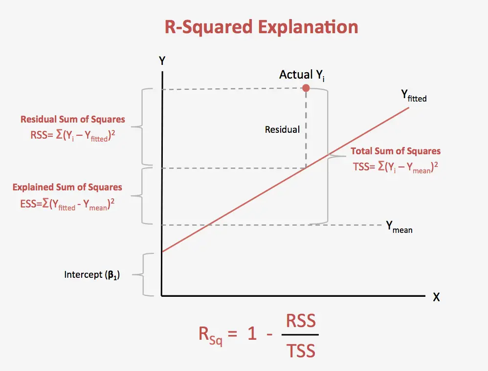
These three quantities are linked by a fundamental identity:

$$\text{TSS}=\text{ESS}+\text{RSS}$$

This equation states that the total variation in $y$ can be perfectly decomposed into the variation explained by the model and the variation that remains unexplained. Proving this identity is the next crucial step.

3. Proof: TSS = ESS + RSS

Your desire for mathematical rigor will be well-served here. The proof is a classic piece of statistical derivation that demonstrates how the properties of OLS lead to this clean decomposition.

We start with the definition of TSS and algebraically manipulate it:

$$\begin{array}{rl}\text{TSS}& =\sum (y_i-\bar{y}{)}^2\\ & =\sum (y_i-{\hat{y}}_i+{\hat{y}}_i-\bar{y}{)}^2\text{(add and subtract }{\hat{y}}_i\text{)}\\ & =\sum [(y_i-{\hat{y}}_i)+({\hat{y}}_i-\bar{y}){]}^2\\ & =\sum (y_i-{\hat{y}}_i{)}^2+\sum ({\hat{y}}_i-\bar{y}{)}^2+2\sum (y_i-{\hat{y}}_i)({\hat{y}}_i-\bar{y})\\ & =\text{RSS}+\text{ESS}+2\sum e_i({\hat{y}}_i-\bar{y})\end{array}$$

The entire proof now hinges on showing that the cross-product term, $\sum e_i({\hat{y}}_i-\bar{y})$, is equal to zero. This is a non-trivial result that follows from the properties of the OLS estimates.

The key steps in the proof that $\sum e_i({\hat{y}}_i-\bar{y})=0$ are:

1. Expand the term: $\sum e_i{\hat{y}}_i-\sum e_i\bar{y}$.
2. The second part, $\bar{y}\sum e_i$, is zero because $\sum e_i=0$.
3. The first part, $\sum e_i{\hat{y}}_i$, is also zero. This is a fundamental property of OLS residuals: they are uncorrelated with the fitted values. The video demonstrates this algebraically. In matrix form, this is because ${\mathbf{e}}^{\prime }\hat{\mathbf{y}}=(\mathbf{My}{)}^{\prime }(\mathbf{Py})={\mathbf{y}}^{\prime }{\mathbf{M}}^{\prime }\mathbf{Py}={\mathbf{y}}^{\prime }\mathbf{MPy}=0$, since the residual-maker matrix $\mathbf{M}$ and projection matrix $\mathbf{P}$ are orthogonal ($\mathbf{MP}=0$).

With the cross-term proven to be zero, the identity $\text{TSS}=\text{ESS}+\text{RSS}$ is established.

4. The Coefficient of Determination ($R^2$)

Now that we have partitioned the total variance, we can define a standardized measure of fit. By dividing the identity $\text{TSS}=\text{ESS}+\text{RSS}$ by TSS, we get:

$$1=\frac{\text{ESS}}{\text{TSS}}+\frac{\text{RSS}}{\text{TSS}}$$

The coefficient of determination, or $R^2$, is defined as the proportion of the total sum of squares that is explained by the model.

$$R^2=\frac{\text{ESS}}{\text{TSS}}$$

Using the identity above, we can also express it as:

$$R^2=1-\frac{\text{RSS}}{\text{TSS}}$$

This second form is often more intuitive: $R^2$ is 1 minus the proportion of variance that is unexplained.

To explore the definition and interpretation of $R^2$ in more detail, let's turn to another resource.

Key properties of $R^2$:

• It is a proportion, so its value ranges from 0 to 1 (assuming the model includes an intercept).
• $R^2=1$: A perfect fit. All variation in $y$ is explained by the model. RSS = 0, meaning all data points lie perfectly on the regression line.
• $R^2=0$: The model has no explanatory power. ESS = 0, which means ${\hat{y}}_i=\bar{y}$ for all $i$. The best prediction for $y$ is simply its average, and the independent variables provide no additional information.
• An $R^2$ of, for example, 0.65 means that 65% of the variance in the dependent variable can be explained by the independent variables in the model.

Test your understanding!

A data scientist fits a simple linear regression model and finds an $R^2$ of 0.70. They believe they can improve the model, so they add five new independent variables and re-fit the regression. The new $R^2$ is 0.75.

Does this increase from 0.70 to 0.75 definitively prove that the second model is a better representation of the underlying relationship between the variables? Why or why not?

Show answer

No, it does not definitively prove the second model is better.

The coefficient of determination, $R^2$, has a mathematical property that it can never decrease when new variables are added to the model. Since RSS is the value being minimized, adding more variables gives the OLS procedure more flexibility to reduce the sum of squared residuals, $\sum e_i^2$. At worst, if a new variable is completely useless, its coefficient will be estimated as zero (or very close to it), and the RSS will remain unchanged. More likely, the model will fit to random noise in the new variables, causing RSS to decrease slightly and $R^2$ to increase, even if the added variables have no true relationship with the dependent variable.

Therefore, the increase from 0.70 to 0.75 might simply be a mathematical artifact of adding more variables, not an indication of a genuinely better model. This phenomenon is a key reason why $R^2$ must be interpreted with caution and why other metrics like Adjusted $R^2$ or techniques like regularization are needed.

Conclusion

In this lesson, we transitioned from analyzing the properties of the OLS estimator to evaluating the performance of the overall regression model.

Key Takeaways:

• Residuals ($e_i=y_i-{\hat{y}}_i$) represent the unexplained error for each observation.
• The total variation in the dependent variable can be decomposed into explained and unexplained parts: TSS = ESS + RSS. This identity is a direct consequence of the properties of OLS.
• The coefficient of determination ($R^2$) is the ratio $\text{ESS}/\text{TSS}$, representing the proportion of variance in $y$ that is explained by the model.
• While useful, $R^2$ has a major limitation: it always increases (or stays the same) when more variables are added, making it a potentially misleading metric for model comparison.

Preview of the Next Lesson:
The tendency of $R^2$ to reward model complexity, even when that complexity is not justified, is a symptom of a larger problem known as overfitting. Our next lesson will introduce a powerful technique to combat this: regularization. We will formulate L2 (Ridge) regularization for linear regression and derive its solution, showing how it penalizes large coefficients to create simpler, more robust models.