Recommended resources
The freely available resources this lesson will direct you to.
Hello! Welcome back to our course.
In the last lesson, we derived Bayes' theorem and explored its use as a formal engine for updating our beliefs about discrete hypotheses in light of new evidence. We saw that this process is central to how systems can "learn" from data. However, many quantities we care about in AI are not simple discrete states but are real-valued numbers—model weights, sensor measurements, or prediction errors.
To handle these, we need to generalize from discrete events to a more powerful concept. This lesson introduces that concept, fulfilling the learning outcome: to define random variables and distinguish between discrete and continuous types. This is a foundational step that bridges the gap between the probability of abstract events and the statistical analysis of numerical data, which is at the heart of machine learning.
1. What is a Random Variable?
At its core, a random variable is a rule that assigns a numerical value to every possible outcome of a random experiment. It provides a way to map the, sometimes abstract, outcomes of an experiment from a sample space, , onto the set of real numbers, .
For example, in an experiment of flipping a coin twice, the sample space is . We could define a random variable, let's call it , to be the number of heads in the outcome.
- For the outcome , assigns the value 2. We write this as .
- For the outcomes and , assigns the value 1. and .
- For the outcome , assigns the value 0. .
This leads to the formal definition:
Definition: A random variable is a function from the sample space to the set of real numbers .

It is crucial to distinguish between the random variable itself (the function, denoted by a capital letter like ) and the numerical values it can take (real numbers, denoted by a lowercase letter like ). The notation is shorthand for "the probability of the set of all outcomes for which ".
To build your intuition on this definition, the following video provides some excellent examples.
5. Discrete Random Variables I
This segment from an MIT OpenCourseWare lecture provides an intuitive introduction to random variables as functions that assign numerical values to experimental outcomes.
Watch from 01:13 to 04:41 and from 09:08 to 11:04. Pay close attention to the distinction made between the random variable as an abstract function (capital letter) and the numerical values it takes (lowercase letter).
2. The Rigorous Definition: Measurability
Your preference for mathematical rigor warrants a deeper look at the formal definition. The statement that a random variable is a "function" is not quite complete. It must be a measurable function.
What does this mean? In our probability space , we can only assign probabilities to sets that are in our -algebra, . For our random variable to be useful, we must be able to ask questions like "What is the probability that takes a value less than or equal to 5?". The set of outcomes that makes this happen is . For the probability of this set to be defined, the set itself must be an element of .
This must hold true not just for "less than 5", but for any "reasonable" set of real numbers (specifically, any set in the Borel -algebra on , denoted ).
Rigorous Definition: Let be a probability space. A function is a random variable if for every set , the preimage of under is in . That is:
This property, called measurability, ensures that is always a well-defined probability.
The following video explains this formal definition very clearly.
Probability Theory 10 | Random Variables
This video from 'The Bright Side of Mathematics' delves into the measure-theoretic definition of a random variable, explaining the crucial property of measurability.
Watch from 00:09 to 07:49. Focus on understanding why the measurability condition is necessary to assign probabilities and how it connects the \sigma-algebra of the sample space to the \sigma-algebra of the real numbers.
For a supplementary text-based explanation, you can refer to the section titled "A more rigorous definition of random variable" in the StatLect article on Random Variables (LINK), which you will be asked to read shortly.
3. Types of Random Variables
Now that we have a solid definition of a random variable, we can classify them. The primary distinction is based on the nature of the set of values the variable can take, known as its support. This leads to two main types: discrete and continuous.
Random variable | Definition, examples, exercises
The following article from StatLect provides concise and clear definitions for the two main types of random variables. It will formalize the concepts we discuss next.
Please read the sections titled 'Types of random variables', 'Discrete random variables', and 'Continuous random variables'. Focus on the definition of support and how it differs for discrete (countable) and continuous (uncountable) variables.
3.1. Discrete Random Variables
As you just read, a random variable is discrete if its support (the set of possible values it can take) is either finite or countably infinite.
- Finite Support Example: Let be the outcome of a standard six-sided die roll. The support is .
- Countably Infinite Support Example: Let be the number of coin flips needed to get the first head. The support is , which is infinite but countable.
For discrete random variables, we can assign a non-zero probability to each individual value in its support. The function that gives this probability, , is called the Probability Mass Function (PMF). We will study this in detail in our next lesson.
3.2. Continuous Random Variables
A random variable is continuous if its support is an uncountable set of real numbers, typically an interval or a union of intervals.
- Example: Let be the exact time it takes for a computer to boot up. can take any value in an interval, say seconds. There are uncountably many possible values in this range.
A critical property of continuous random variables is that the probability of the variable taking on any single specific value is zero. That is, for any continuous random variable and any value , .
This might seem paradoxical, but it makes sense if you consider that there are infinitely many points in any interval. Instead of asking about the probability of a single point, we ask about the probability of the variable falling within an interval. This probability is found by integrating a function called the Probability Density Function (PDF), which we will explore in a future lesson.
4. Summary and Comparison
The distinction between discrete and continuous random variables is fundamental. The following table summarizes their key differences.
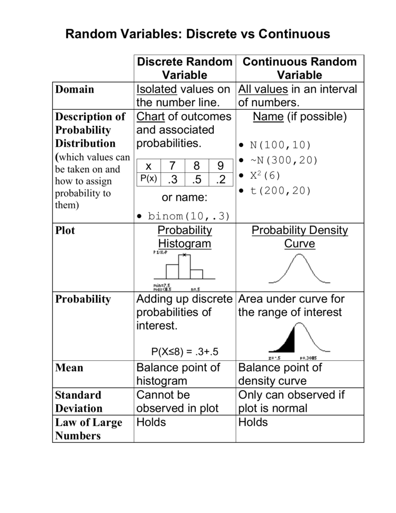
Test your understanding!
Classify each of the following random variables as either discrete or continuous.
- : The number of emails arriving in your inbox in one hour.
- : The exact weight of a randomly selected apple from a batch.
- : The number of defective pixels on a new computer monitor.
- : The voltage of a battery, measured with infinite precision.
- : The number of steps you take in a day.
Show answer
- Discrete. The number of emails must be a non-negative integer (0, 1, 2, ...). The support is countably infinite.
- Continuous. Weight can take any real value within a certain range (e.g., between 100g and 300g). The support is an interval.
- Discrete. The number of defective pixels is a non-negative integer. The support is finite (up to the total number of pixels on the screen).
- Continuous. Voltage, measured with infinite precision, can take any real value within the battery's operating range.
- Discrete. The number of steps is a non-negative integer. The support is countable.
Conclusion
In this lesson, we established the formal definition of a random variable as a measurable function that maps outcomes from a sample space to the real numbers. This provides the crucial link between abstract probability theory and the numerical data we work with in machine learning.
Key Takeaways:
- A random variable is a function .
- The measurability property is required to ensure that we can calculate probabilities for events like .
- Random variables are classified based on their support (the set of values they can take).
- Discrete random variables have a finite or countable support. We can assign a non-zero probability to each specific value.
- Continuous random variables have an uncountable support (like an interval). The probability of the variable equaling any single specific value is always zero.
Preview of the Next Lesson:
Now that we have clearly defined discrete random variables, we need a way to describe their behavior fully. In the next lesson, we will formally define and compute Probability Mass Functions (PMFs), which provide a complete probabilistic description of a discrete random variable.