Probability Rules: Addition, Multiplication, and Conditional Probability

Hello! Welcome to your next lesson in the Foundations of Probability Theory.

In our last session, we established the rigorous axiomatic foundation for probability. We defined the probability space as a triplet $(\Omega ,\mathcal{F},P)$ and showed how all basic properties, such as $P(A^c)=1-P(A)$, can be derived directly from Kolmogorov's three axioms.

Today, we will build on that foundation to derive and apply the essential rules for calculating probabilities in more complex scenarios. These rules—the addition rule, the multiplication rule, and the concept of conditional probability—are the practical workhorses of probability theory. Your goal for this lesson is to apply probability rules including addition, multiplication, and conditional probability. Mastering these will allow you to solve a wide range of problems by breaking them down into simpler, sequential parts.

1. The Addition Rule for Non-Disjoint Events

From the axioms, we know that for any two disjoint (mutually exclusive) events $A$ and $B$, the probability of their union is simply the sum of their probabilities: $P(A\cup B)=P(A)+P(B)$.

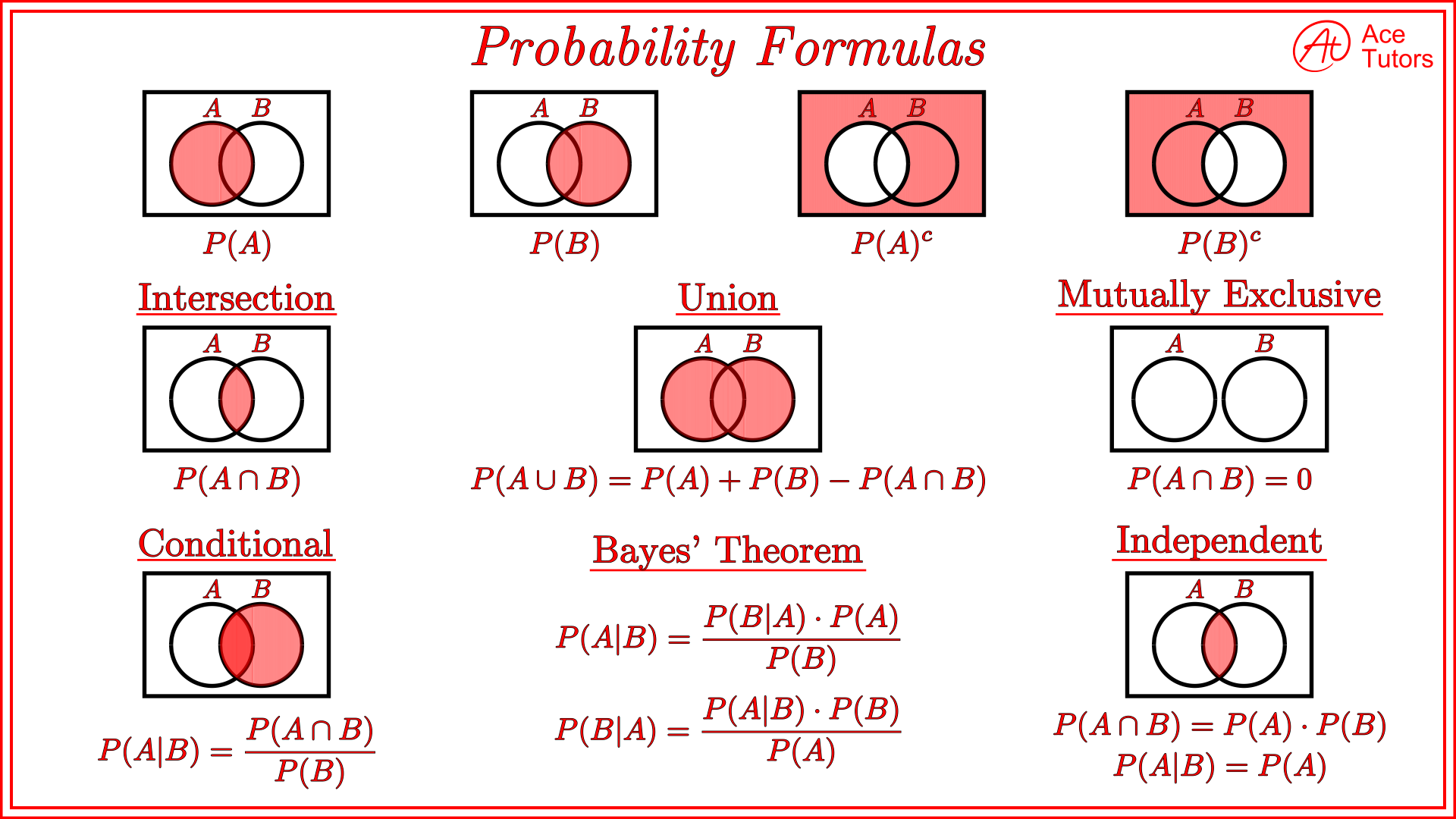
But what if the events are not disjoint? What if they can both occur, meaning $A\cap B\ne \varnothing$? If we simply add $P(A)$ and $P(B)$, we double-count the probability of the intersection, $P(A\cap B)$. The general addition rule, also known as the principle of inclusion-exclusion for two events, corrects for this.

As you saw, the proof relies on decomposing the union $A\cup B$ into disjoint sets. Let's formalize that argument, as you appreciate the rigorous details:

1. We can express the union $A\cup B$ as the union of two disjoint sets: $A$ and the part of $B$ that is not in $A$, which is $B\cap A^c$. So, $A\cup B=A\cup (B\cap A^c)$.
2. By Axiom 3 (Additivity), $P(A\cup B)=P(A)+P(B\cap A^c)$.
3. We also know that event $B$ can be decomposed into two disjoint parts: the part in $A$ ($B\cap A$) and the part not in $A$ ($B\cap A^c$). So, $B=(B\cap A)\cup (B\cap A^c)$.
4. By Axiom 3 again, $P(B)=P(B\cap A)+P(B\cap A^c)$.
5. Rearranging this gives $P(B\cap A^c)=P(B)-P(B\cap A)$.
6. Substituting this back into our equation from step 2, we get:
   $P(A\cup B)=P(A)+P(B)-P(A\cap B)$

This rule is fundamental for calculating the probability of "at least one" of two events occurring.

2. Conditional Probability: Updating Beliefs

Often, we need to update our assessment of an event's probability based on new information. The mathematical formalism for this is conditional probability. We denote the probability of event $A$ occurring given that event $B$ has occurred as $P(A|B)$.

The core idea is that observing event $B$ restricts our sample space. Outcomes outside of $B$ are no longer possible. We are now working within the "world" of $B$, and we need to re-normalize our probabilities to reflect this new, smaller universe.

The formal definition of the conditional probability of $A$ given $B$ is:
$P(A|B)=\frac{P(A\cap B)}{P(B)},\text{provided that }P(B)>0$
This definition is one of the most important in all of probability theory.

3. The Multiplication Rule and Independence

By rearranging the definition of conditional probability, we arrive at the multiplication rule, which is essential for calculating the probability of the intersection of events (i.e., that they both happen).
$P(A\cap B)=P(A|B)P(B)$
This rule is incredibly useful because it allows us to model sequential experiments. We can think of it as: "The probability of A and B happening is the probability of B happening, multiplied by the probability of A happening, given that B has already happened."

Independence

A crucial special case arises when the occurrence of event $B$ provides no information about the probability of event $A$. In this case, we say the events are independent.

Formally, events $A$ and $B$ are independent if and only if:
$P(A\cap B)=P(A)P(B)$
If $P(B)>0$, this is equivalent to $P(A|B)=P(A)$. This provides the intuitive meaning: knowing $B$ happened doesn't change the probability of $A$.

The multiplication rule can be generalized to a sequence of $n$ events. This is often called the chain rule of probability. As you saw briefly at the end of the video on conditional probability (LINK), for events $A_1,A_2,\dots ,A_n$:
$P(A_1\cap \cdots \cap A_n)=P(A_1)P(A_2|A_1)P(A_3|A_1\cap A_2)\dots P(A_n|A_1\cap \cdots \cap A_{n-1})$
This powerful rule is the foundation for many models in machine learning, such as language models and Bayesian networks.

Test your understanding!

A standard 52-card deck is shuffled. You draw one card. Let $A$ be the event that the card is a King, and let $B$ be the event that the card is a "face card" (Jack, Queen, or King). Are events $A$ and $B$ independent? Prove your answer using the definition of independence.

Show answer

To check for independence, we must verify if $P(A\cap B)=P(A)P(B)$.

1. Calculate $P(A)$: There are 4 Kings in a 52-card deck. So, $P(A)=\frac{4}{52}=\frac{1}{13}$.

2. Calculate $P(B)$: There are 3 face cards (J, Q, K) in each of the 4 suits. So, there are $3\times 4=12$ face cards. $P(B)=\frac{12}{52}=\frac{3}{13}$.

3. Calculate $P(A\cap B)$: The event "A and B" means the card is both a King and a face card. Since all Kings are face cards, this intersection is just the event $A$. So, $A\cap B=A$, and $P(A\cap B)=P(A)=\frac{4}{52}=\frac{1}{13}$.

4. Check for independence: We compare $P(A\cap B)$ with $P(A)P(B)$.
   $P(A)P(B)=\left(\frac{1}{13}\right)\left(\frac{3}{13}\right)=\frac{3}{169}$
   Since $P(A\cap B)=\frac{1}{13}$ and $P(A)P(B)=\frac{3}{169}$, these are not equal.

Therefore, the events $A$ and $B$ are dependent. This makes intuitive sense: knowing a card is a face card increases its probability of being a King.

4. Application: The Newton-Pepys Problem

Let's see these rules in action in a classic problem posed to Isaac Newton in 1693. Which of the following three events is most likely?

• Event A: Getting at least one 6 when six fair dice are rolled.
• Event B: Getting at least two 6s when twelve fair dice are rolled.
• Event C: Getting at least three 6s when eighteen fair dice are rolled.

This is a non-trivial problem that requires the careful application of the rules we've learned, particularly the complement rule and the multiplication rule for independent events.

Let's re-examine the calculation for $P(A)$:

• Calculating the probability of "at least one 6" directly would require using the inclusion-exclusion principle for 6 events, which is very complicated.
• It's much easier to calculate the probability of the complement event, $A^c$, which is "getting no 6s".
• The rolls of the six dice are independent. The probability of not getting a 6 on any single die is $\frac{5}{6}$.
• Using the multiplication rule for independent events, the probability of getting no 6s on all six dice is:
  $P(A^c)=\left(\frac{5}{6}\right)\times \left(\frac{5}{6}\right)\times \cdots \times \left(\frac{5}{6}\right)={\left(\frac{5}{6}\right)}^6$
• Finally, using the complement rule:
  $P(A)=1-P(A^c)=1-{\left(\frac{5}{6}\right)}^6\approx 0.665$

As the video shows, repeating this logic reveals that Event A is the most likely, contrary to many people's initial intuition.

Conclusion

In this lesson, we have moved from the abstract axioms of probability to the concrete rules used for calculation. You have seen how these rules are not arbitrary but are rigorously derived from the foundational axioms.

Key Takeaways:

• General Addition Rule: For any two events $A$ and $B$, $P(A\cup B)=P(A)+P(B)-P(A\cap B)$.
• Conditional Probability: The probability of $A$ given $B$ is $P(A|B)=\frac{P(A\cap B)}{P(B)}$, representing an update of belief based on new information.
• Multiplication Rule: For any two events $A$ and $B$, $P(A\cap B)=P(A|B)P(B)$.
• Independence: Events $A$ and $B$ are independent if $P(A\cap B)=P(A)P(B)$, which is equivalent to $P(A|B)=P(A)$.

Preview of the Next Lesson:
The rules we learned today are all that is needed to derive one of the most celebrated and useful results in probability: Bayes' Theorem. In the next lesson, we will derive and apply Bayes' theorem for updating beliefs. You will see that while its derivation is a simple algebraic step, its application provides a powerful engine for inference and learning in the face of uncertainty.